

Abstract
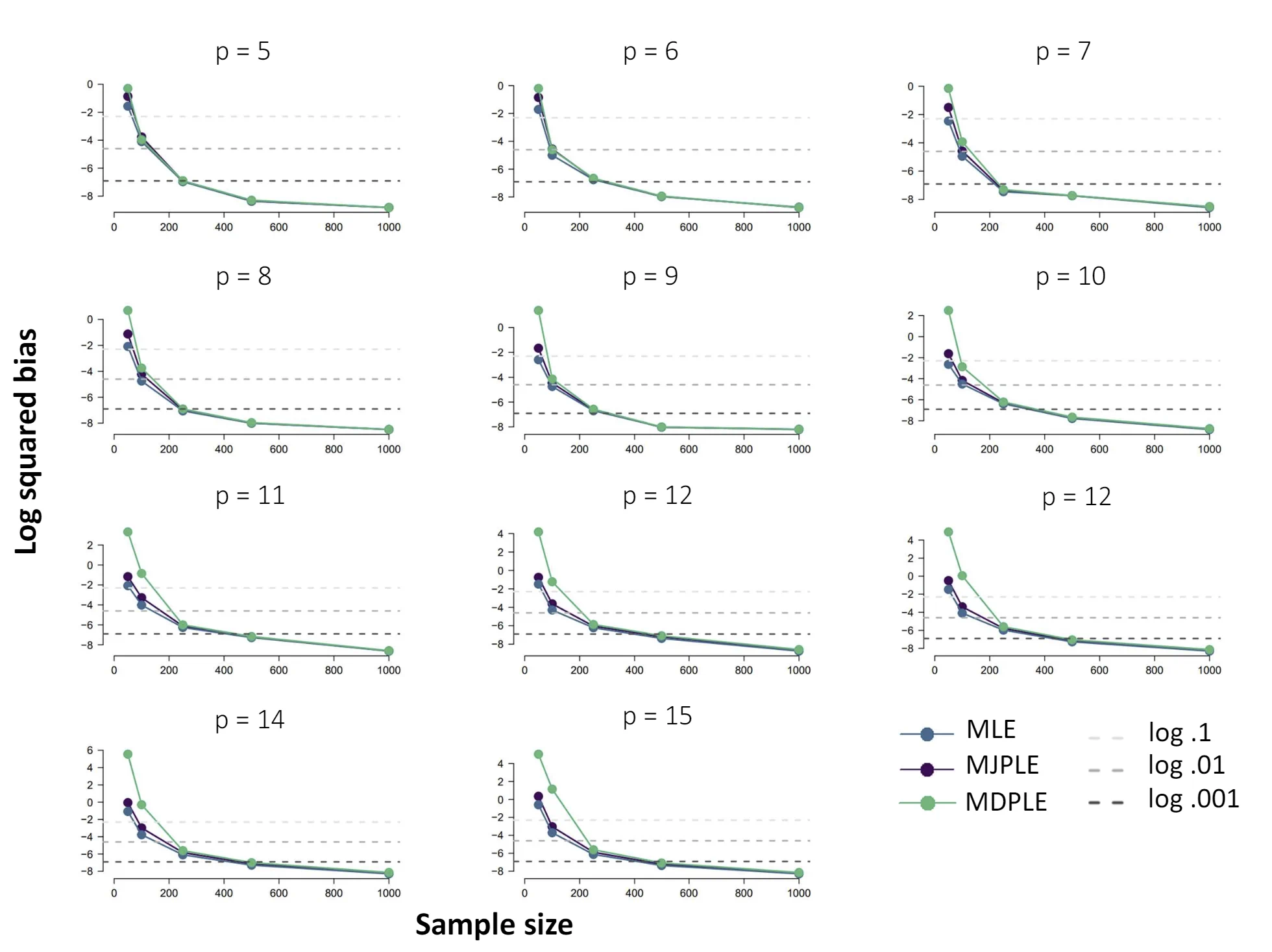
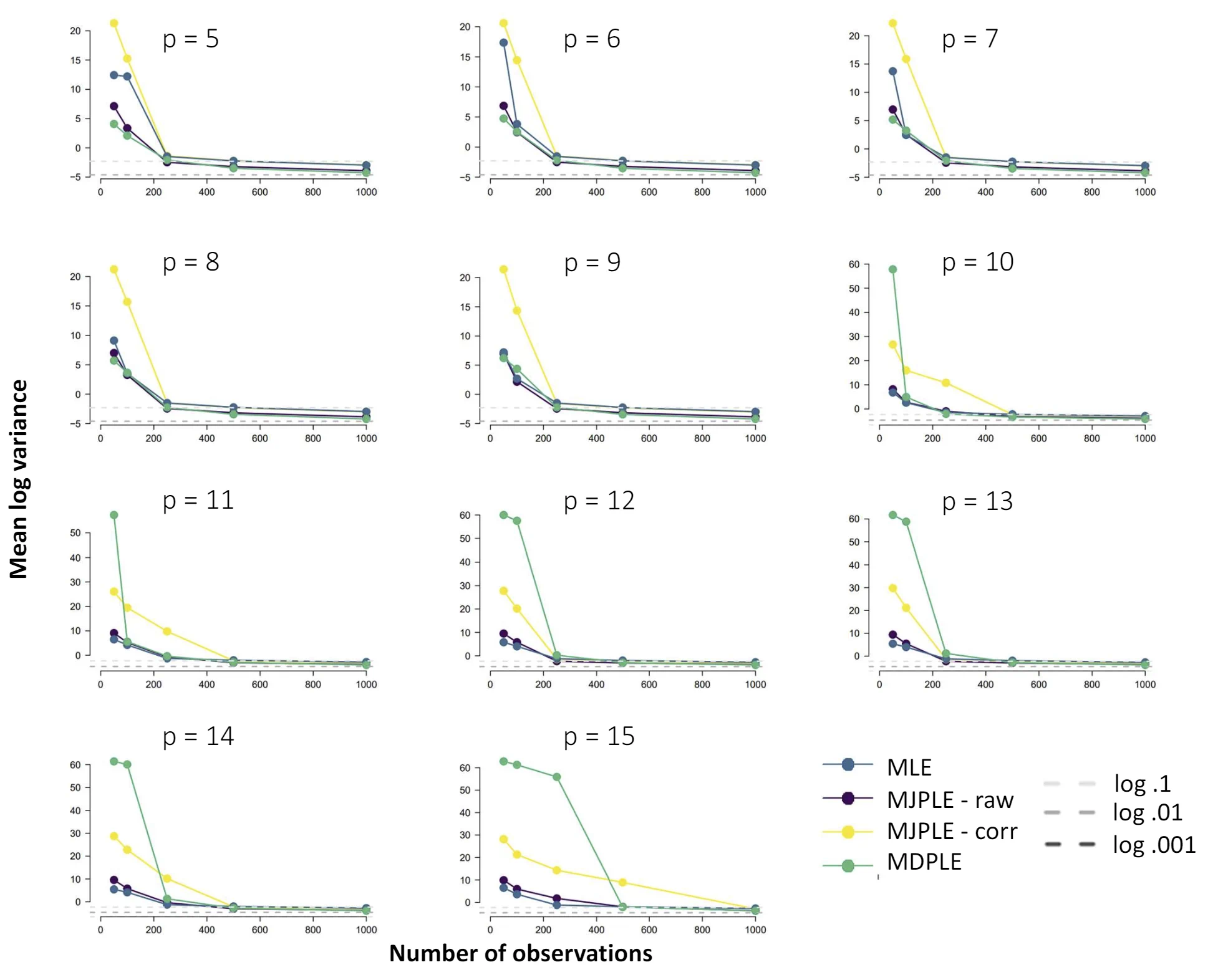
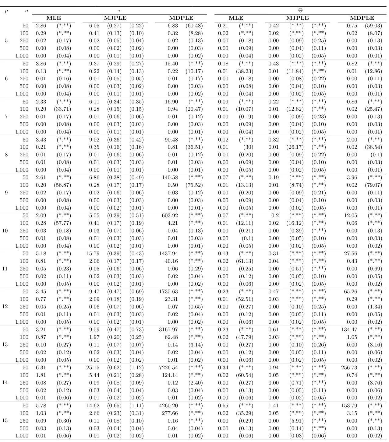
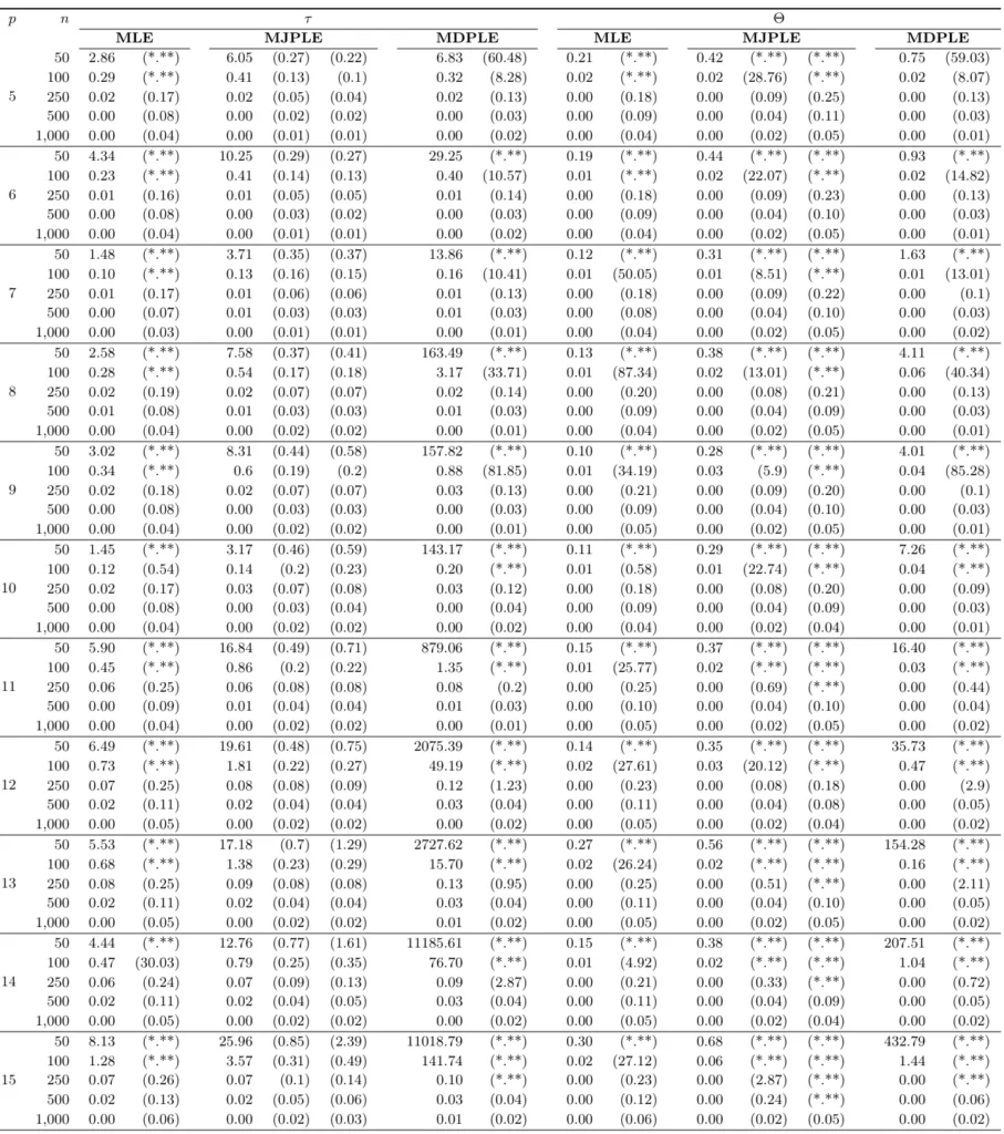
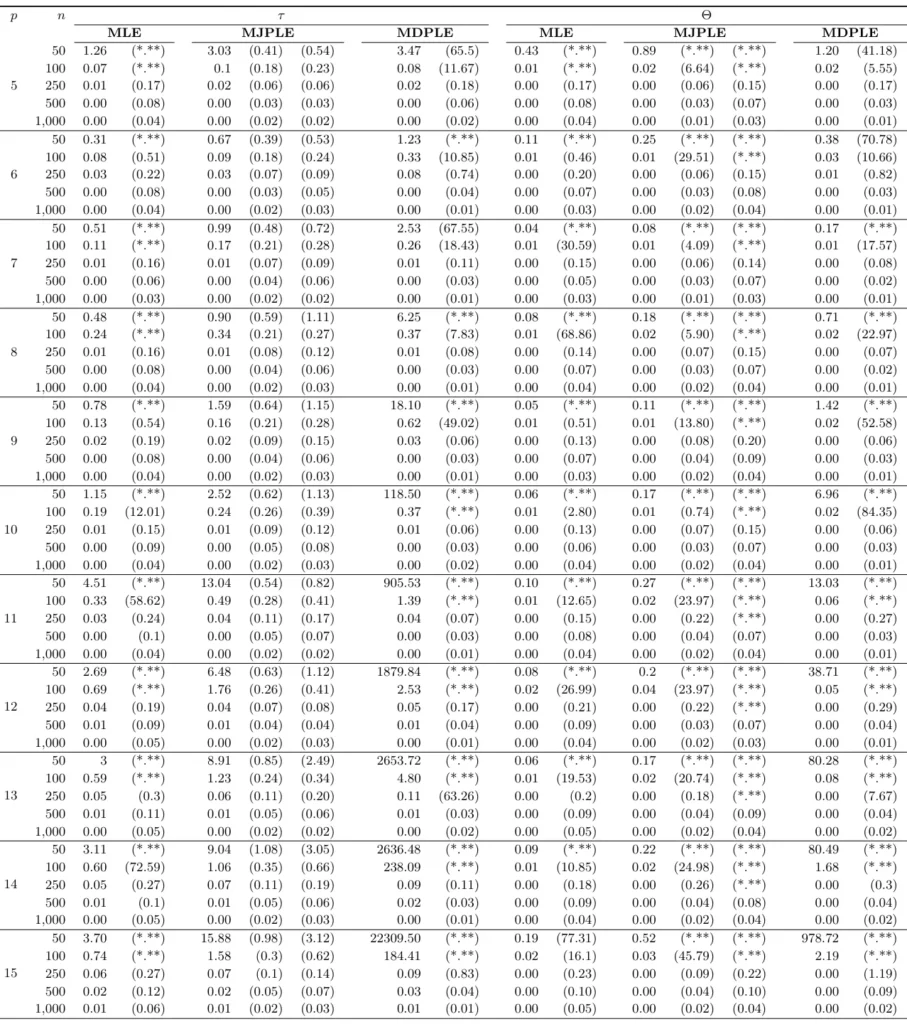
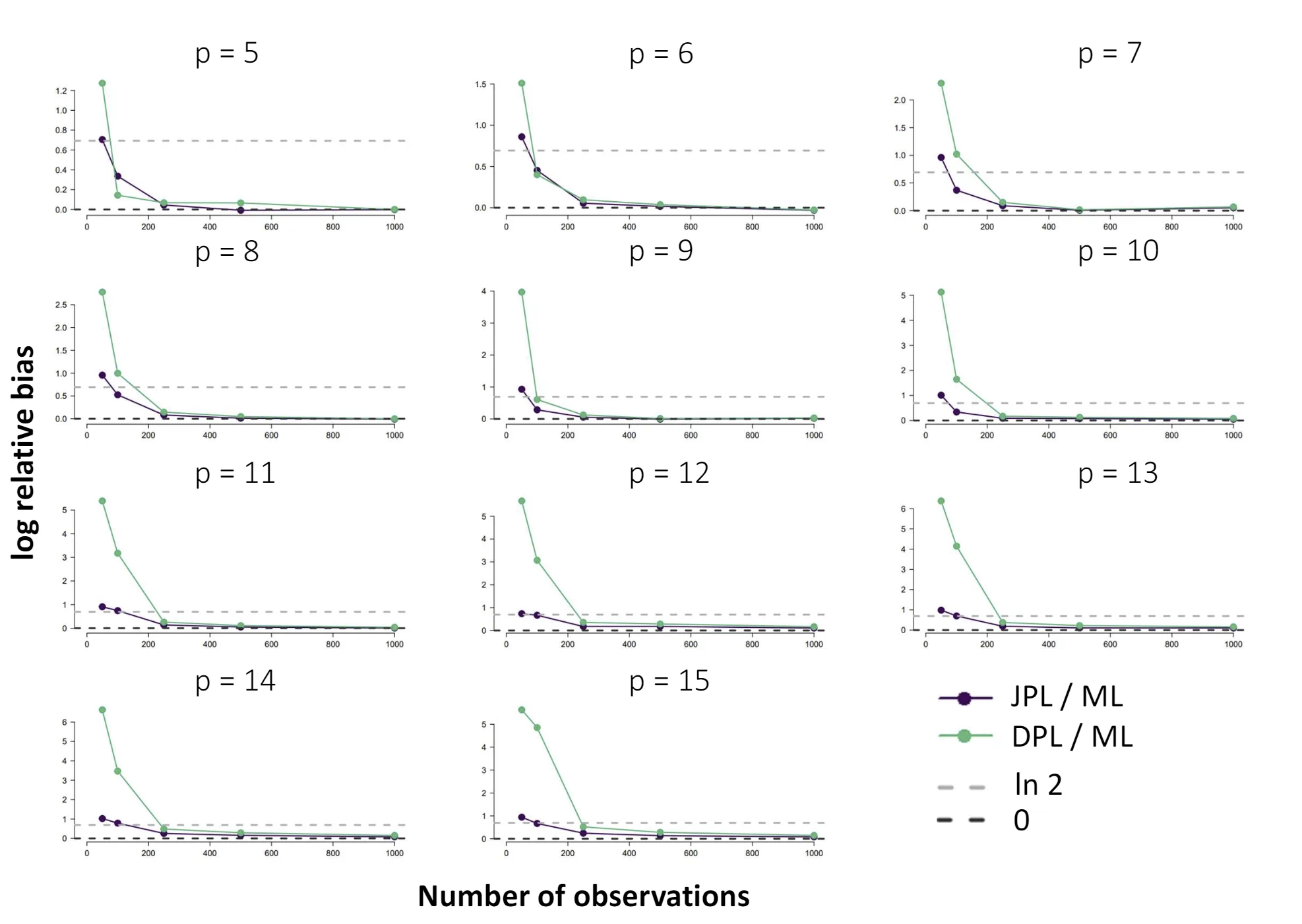
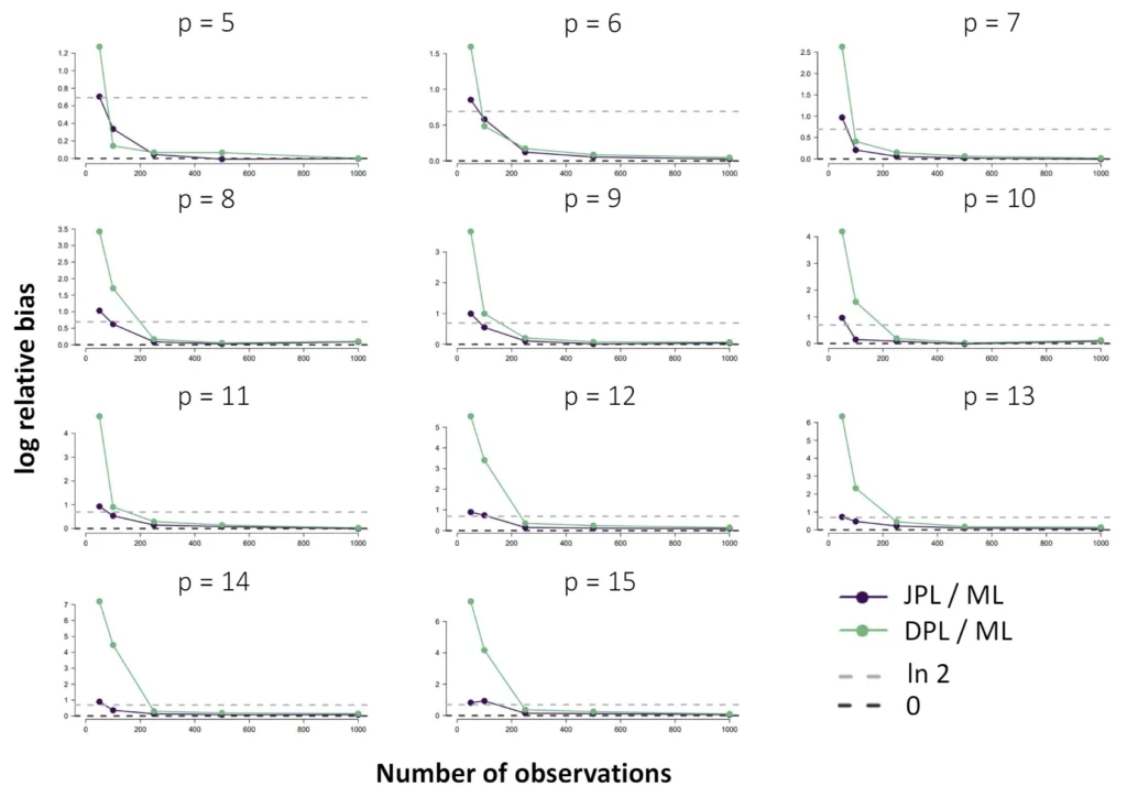
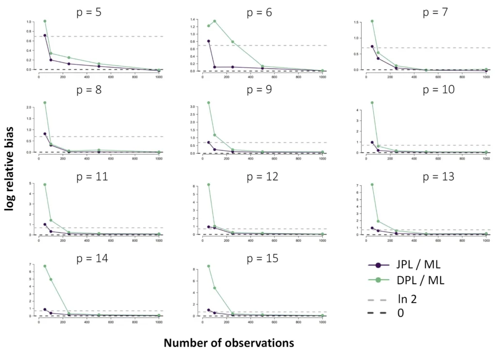
The Ising model is one of the most popular models in network psychometrics. However, statistical analysis of the Ising model is difficult due to the presence of its intractable normalizing constant in the probability function. As a result, maximum likelihood estimation using the exact likelihood is only possible for small graphs, and approximation methods are needed for larger graphs. Two popular approximations of the exact likelihood are the joint pseudolikelihood (JPL) and the disjoint pseudolikelihood (DPL). These approximations yield consistent estimators, but we do not know how well they perform for finite data. In this paper, we investigate the relative performance of parameter estimation methods based on the two approximations and compare them to maximum likelihood estimation using the exact likelihood. We perform an extensive simulation study comparing the estimators in terms of bias and variance. We show that maximum pseudolikelihood estimation based on the JPL is a stable estimation method that is able to accurately approximate the maximum likelihood estimates, but that maximum pseudolikelihood estimation based on the DPL only works well for large sample sizes.
Editor Curated
Key Takeaways
- While Maximum Likelihood (ML) estimation is the most accurate method for the Ising model in network psychometrics, it is only computationally feasible for small graphs.
- For larger graphs, Maximum Pseudolikelihood (MPL) estimators, specifically the Joint (JPL) and Disjoint (DPL) pseudolikelihoods, offer consistent and viable alternatives.
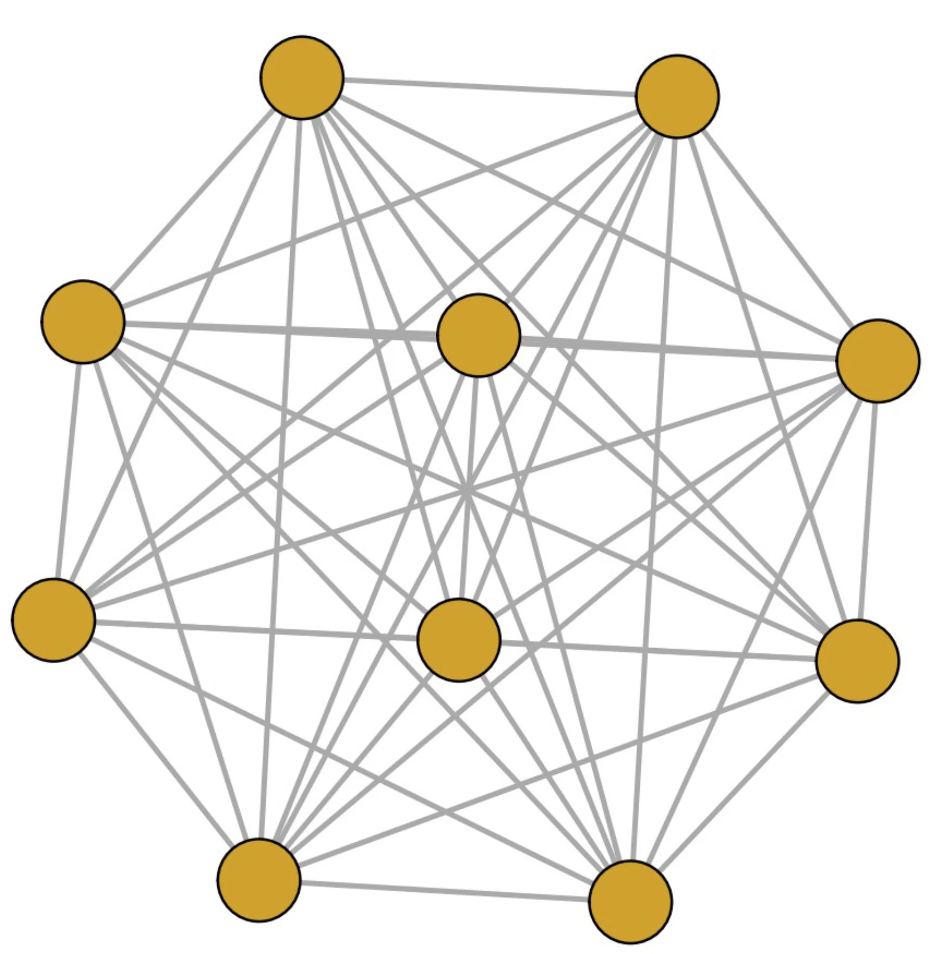
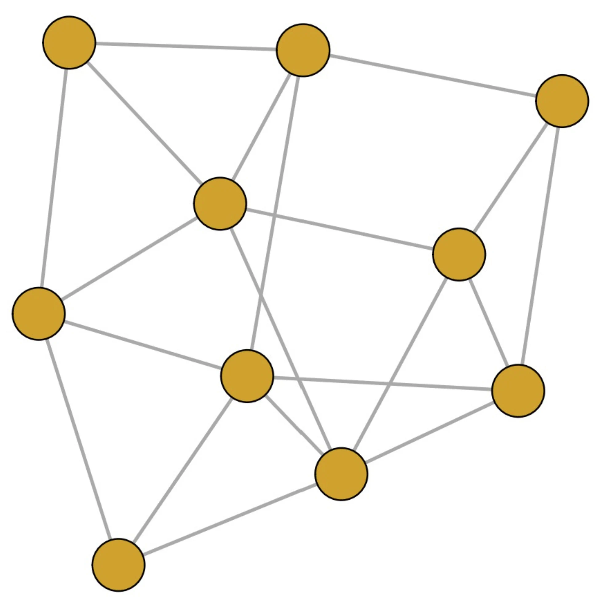
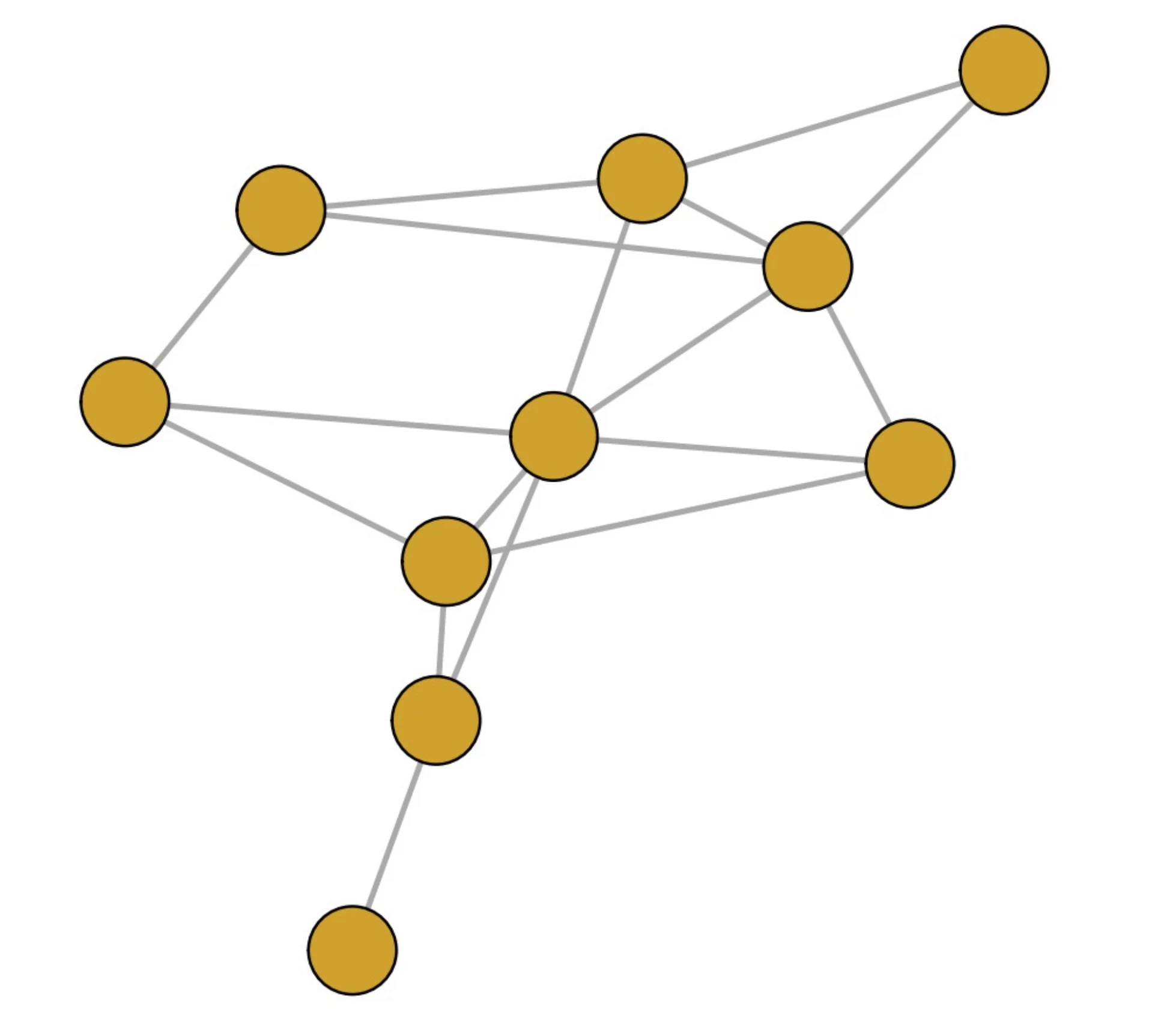
- The choice between these alternatives depends on the network's structure; simulations show that the DPL is more efficient for sparse networks, while the JPL performs better for dense networks.
Keywords: