Discovering cyclic causal models in psychological research

Kyuri Park1*, Lourens J. Waldorp2, & Oisín Ryan3

Received: June 1, 2023. Accepted: April 15, 2024. Published: April 22, 2024. https://doi.org/10.56296/aip00012

Abstract
Statistical network models have become popular tools for analyzing multivariate psychological data. In empirical practice, network parameters are often interpreted as reflecting causal relationships – an approach that can be characterized as a form of causal discovery. Recent research has shown that undirected network models are likely to perform poorly as causal discovery tools in the context of discovering acyclic causal structures, a task for which many alternative methods are available. However, acyclic causal models are likely unsuitable for many psychological phenomena, such as psychopathologies, which are often characterized by cycles or feedback loop relationships between symptoms. A number of cyclic causal discovery methods have been developed, largely in the computer science literature, but they are not as well studied or widely applied in empirical practice. In this paper, we provide an accessible introduction to the basics of cyclic causal discovery for empirical researchers. We examine three different cyclic causal discovery methods and investigate their performance in typical psychological research contexts by means of a simulation study. We also demonstrate the practical applicability of these methods using an empirical example and conclude the paper with a discussion of how the insights we gain from cyclic causal discovery relate to statistical network analysis.

Keywords: constraint-based, cyclic causal discovery, directed cyclic graph (DCG), partial ancestral graph (PAG), statistical network model

  1. Computational Science Lab, Informatics Institute, University of Amsterdam
  2. Department of Psychology, University of Amsterdam
  3. Department of Data Science and Biostatistics, Julius Centre, University Medical Centre Utrecht

*Please address correspondence to kyurheep@gmail.com, Computational Science Lab, Informatics Institute, Faculty of Science, University of Amsterdam, PO Box 94323, 1090 GH Amsterdam, The Netherlands

Park, K., Waldorp, L. J., & Ryan, O. (2024). Discovering cyclic causal models in psychological research. advances.in/psychology, 2, e72425. https://doi.org/10.56296/aip00012

The current article passed two rounds of double-blind peer review. The anonymous review report can be found here.


Introduction

A fundamental task in various disciplines of science is to understand the mechanisms or causal relations underlying the phenomena of interest. In psychology, one of the core questions is how psychopathology comes about, with the network theory positing that mental disorder is produced by a system of direct causal interactions between symptoms (Borsboom & Cramer, 2013). Given this theoretical framework, statistical network models have become popular tools for analyzing multivariate observational data (Robinaugh et al., 2020; Epskamp et al., 2018a). In practice, empirical researchers often interpret the conditional statistical relationships estimated in a network model as reflecting the causal relationships between symptoms of mental disorder and/or other psychological variables — an approach that can be characterized as a form of causal discovery (Spirtes et al., 2000; Peters et al., 2017; Ryan et al., 2022). However, it has been shown that network models are likely to perform poorly as causal discovery tools; relations in the network may not reflect the direct causal effects that researchers aim to discover, as they may be produced by, amongst other inferential issues, unwittingly conditioning on common effects (Dablander & Hinne, 2019; Ryan et al., 2022).

In the field of causal discovery, one class of methods that utilizes patterns of statistical (in)dependence estimated from observational data to infer causal structures is known as constraint-based causal discovery (Spirtes & Glymour, 1991). Ryan et al. (2022) suggest that network models could be replaced by purpose-built constraint-based causal discovery methods. However, the most popular and well-studied constraint-based methods assume that causal relationships are acyclic; that is if X causes Y, then Y does not cause X (Glymour et al., 2019). Although so-called Directed Acyclic Graphs (DAGs) (Pearl, 2009) are popular tools for causal modeling (Tennant et al., 2021), the acyclicity assumption is problematic when studying a phenomena such as mental disorders, since cyclic relationships or feedback loops are critical to the theoretical understanding of psychopathology (Borsboom, 2017; Haslbeck et al., 2021). For example, Wittenborn et al. (2016) suggest that several different causal feedback loops, such as perceived stress negative affect rumination perceived stress play a key role in sustaining depression. Such theoretical expectations necessitate the use of cyclic causal discovery methods.

Although some constraint-based cyclic causal discovery algorithms have been developed (Mooij & Claassen, 2020; Richardson, 1996a; Strobl, 2019), they have not been as well studied as their acyclic counterparts. In part, this is due to the conceptual and practical difficulties in fitting and interpreting cyclic causal models. Conceptually, a number of researchers in the causal modeling literature have shown that, under certain conditions, cyclic causal models fit to cross-sectional data may be interpreted as reflecting causal relations between equilibriums or resting states of a dynamic system (Iwasaki & Simon, 1994; Dash, 2005; Strotz & Wold, 1960; Spirtes, 1995; Mooij et al., 2013; Weinberger, 2021; Bongers et al., 2022). From this perspective, cyclic causal relations should be interpreted as a kind of coarse-grained or time-averaged representation of (reciprocal) causal relations between processes that evolve over time; for a detailed treatment of cyclic equilibrium causal models in the context of psychological modeling, we refer readers to Ryan and Dablander (2022). On the practical side, in the context of structural equation modeling, it is well known that all acylic path-models (i.e. containing independent error terms and no latent variables) are statistically identified, whereas this is not generally the case for path models which contain cycles (Bongers et al., 2021; Bollen, 1989). Furthermore, interpreting the output of cyclic causal discovery algorithms is significantly more challenging than for their acyclic counterparts: Even in ideal scenarios, the same pattern of statistical dependence that can be used to deduce a direct causal link in a DAG may not reflect a direct causal link in a cyclic graph (Bongers et al., 2018; Hyttinen et al., 2013). Recent work has explored the application of invariance-based algorithms — another type of causal discovery methods capable of estimating cycles — to psychological data (Kossakowski et al., 2021). However, these methods require multiple datasets that measure the same variables but in different settings, such as a mix of observational and experimental data, which is a disadvantage compared to constraint-based methods that can be applied using only a single observational dataset (Peters et al., 2016; Glymour et al., 2019).

To our knowledge, little research has been done on the applicability of constraint-based cyclic causal discovery methods in psychology, and much remains unknown about their performance. Therefore, in this paper, we aim to address the following question: How well do constraint-based cyclic causal discovery methods perform in typical psychological research contexts? First, we will provide an accessible overview of the different cyclic causal discovery methods, including the assumptions under which they are expected to work and how the output of these methods should be interpreted. Second, we investigate, by means of a simulation study, how well these different methods perform under various circumstances. In the simulation study, we study more and less ideal situations, by varying the sample size, the size and density of the underlying network, and the presence or absence of unobserved confounding variables. Third, we demonstrate the practical applicability of these methods by applying them to empirical data (McNally et al., 2017) and discussing how the insights we gain relate to the statistical network analysis of the same data.

Background

In this section, we will establish the basic concepts of graphical models and examine how constraint-based causal discovery methods operate. We will first introduce different types of graphical models, while demonstrating the differences between statistical and causal graphical models using example graphs. Then, we will explain the assumptions that underlie constraint-based causal discovery methods, as well as the technical difficulties that arise in the presence of cycles. Lastly, we will illustrate each step of the constraint-based causal discovery procedure using a simple example of a directed graph.

Graphical Models

 A graph is a pair \(\mathcal{G} = (\mathcal{V}, \mathcal{E})\), where \(\mathcal{V}\) is a set of vertices and \(\mathcal{E}\) is a set of edges, describing the connections between the vertices. A probabilistic graphical model uses a graph to express the conditional (in)dependencies between random variables, where the vertices represent random variables, and the edges encode the conditional dependencies that hold among the set of variables (Lauritzen, 1996).

There exist various graphical models that differ in the types of edges they allow (e.g., directed vs. undirected) and how edges are interpreted in terms of statistical relationships. One commonly known graphical model in psychology is the Pairwise Markov Random Field (PMRF) — an undirected graph where edges indicate a statistical association between variables after controlling for all other variables — which forms the basis of statistical network models such as the Gaussian Graphical Model (GGM) (Epskamp et al., 2018b; Epskamp & Fried, 2018). In PMRFs, edges are strictly undirected, and the presence of an edge A − B indicates that A and B are statistically dependent, conditional on the set of all other variables in the network (Borsboom et al., 2021). Models like the GGM and Ising network model can be seen as parameterizations of the PMRF. These models assume particular distributions for the variables involved, and, in the case of the GGM, assume that conditional (in)dependence relations can be captured by linear dependence parameters such as the partial correlation.

In a causal graphical model, on the other hand, the edges describe causal relationships between variables; the edges are typically directed, with A B denoting that intervening on A results in a change in the probability distribution of B (Geiger & Pearl, 1990). The simplest and most commonly used causal graph is a directed acyclic graph (DAG), which is commonly utilized to represent a Bayesian network. A DAG consists of directed edges without any cycles (Pearl, 1988). When a causal graph contains cycles, it is referred to as a directed cyclic graph (DCG). Two examples of causal graphical models are shown in Figure 1. Figure 1(a) does not contain any cycles, whereas Figure 1(b) does; hence they are called a DAG and DCG, respectively. In Figure 1(b), the cycle X2X3 denotes that X2 is a direct cause of X3 and X3 is a direct cause of X2.

Figure 1

Example causal graphical models and corresponding PMRF models.

Illustration of example causal graphical models and corresponding pairwise Markov random field (PMRF) models in psychological research.
Note. (a) is the example directed acyclic graph (DAG). (b) is the example directed cyclic graph (DCG). (c) is the PMRF (Pairwise Markov Random Field) corresponding to the DAG in (a). (d) is the PMRF corresponding to the DCG in (b).

Causal graphical models also describe patterns of statistical independencies, which can be read off from structure of the graph using Pearl’s d-separation criterion (Geiger et al., 1990). The idea of this criterion is to associate dependence with connectedness (i.e., the path between A and B is activated by C; d-connected by C) and independence with separation (i.e., the path between A and B is blocked by C, and so these variables are d-separated by C; for a detailed formal treatment of d-separation, see Tian et al., 1998). Formally, two variables A and B are said to be d-separated given C if and only if all paths between A and B are blocked when conditioning on C (Pearl, 2009). Different types of directed paths in a graph are either blocked or unblocked by conditioning on variables along them. For instance, in Figure 1(a), we see a chain structure X1 X2 X3, which implies that X1 and X3 are marginally dependent (X1 \(\not\!\perp\mkern-10mu\perp\)X3) but independent conditional on X2 (X1 \(\perp\mkern-10mu\perp\)X3 | X2). More formally, we would say X1 and X3 are d-connected given the empty set but d-separated by X2. A fork structure X3X2 X4 implies the same pattern of independencies; X3 and X4 are marginally dependent (X3 \(\not\!\perp\mkern-10mu\perp\)X4) but independent conditional on X2 (X3 \(\perp\mkern-10mu\perp\)X4 | X2). However, a collider structure X2X4X5 implies a contrasting pattern; here X2 and X5 are marginally independent (i.e., d-separated when conditioning on the empty set, X2 \(\perp\mkern-10mu\perp\)X5) but dependent conditional on X4 (X2 \(\not\!\perp\mkern-10mu\perp\)X5 | X4). This distinguishing characteristic of colliders is crucial when identifying the directions of causal relationships, as will be shown in Section 2.3. In principle, the d-separation criterion can be applied to both acyclic and cyclic causal graphs, as long as certain conditions, discussed in Section 2.2, are met.

Having established the basics, we can now examine how PMRF-based statistical network models relate to different types of directed causal models. In Figure 1(c), we show the PMRF model that corresponds to the DAG in Figure 1(a), where an additional edge is introduced between X2X5 due to conditioning on the common effect (i.e., collider), X4. In Figure 1(d), the PMRF model corresponding to the DCG in Figure 1(b) is shown. Two spurious edges are induced in the PMRF network (e.g., X1X3 and X2X4) because of conditioning on the colliders X2 and X3. These examples illustrate the limitations of statistical network models in inferring patterns of directed causal relationships. PMRFs can contain spurious edges resulting from conditioning on common effects, and the possibility of producing collider structures is likely to be higher with the presence of cycles, exacerbating this issue. Notably, while the mapping from a causal graph to the statistical network we show here is unique, the two statistical networks presented may have been generated by various distinct causal graphs, including those with or without cycles. For more details on the relationship between PMRF-based networks and causal graphs, we refer readers to Ryan et al. (2022).

Despite this limitation, in practice, PMRFs have often been interpreted as a causal skeleton — the undirected version of a causal graph (Haslbeck & Waldorp, 2018). Further elaborating on this, Ryan et al. (2022) demonstrated how PMRF-based network models can, in fact, be used to identify a so-called equivalence class of causal graphs under certain assumptions. However, these models are prone to suboptimal performance, as the equivalence class they identify is likely much larger than that of custom-built causal discovery methods. Consequently, the authors suggest that causal discovery methods specifically designed for this task are likely to outperform statistical network models in learning the underlying causal structure, indicating that network models may not be desirable tools for discovering causal relationships. In the following sections, we will focus on how constraint-based causal discovery methods recover the causal structure while looking into the assumptions they require. Additionally, we will explore the practical and conceptual difficulties involved in performing causal discovery in the presence of causal cycles.

Acyclic vs. Cyclic Causal Graphs

The d-separation criterion described above applies to all acyclic graphs, but for graphs with cycles, it applies only under certain conditions. To understand these conditions, we first need to introduce some graph terminology. In the field of graphical models, we use kinship terminology to describe a graph structure, as follows:

Acyclic vs. Cyclic Causal Psychometric Network Graphs

Also, when there exists an edge between two vertices A B, A and B are said to be adjacent. For example, in Figure 1(b), X1paG(X2), X2chG(X1), {X1, X2, X3, X4} ∈ anG(X3), {X1, X2, X3} ∈ deG(X1), and X2 is adjacent to X1 and X3. With this terminology in place, we can define the conditions that relate patterns of causal dependency in a causal graph to patterns of statistical dependency between random variables. First, we introduce the global Markov condition, which states that d-separation relations represented in causal graphs can be used to read off statistical independence relations such that:

if XA \(\perp\mkern-10mu\perp\)G XB | XC XA \(\perp\mkern-10mu\perp\) XB | XC for all disjoint subsets of XA, XB, XC,

where \(\perp\mkern-10mu\perp\)G refers to d-separation in graphs, and \(\perp\mkern-10mu\perp\) refers to statistical independence between random variables. If causal graphs are acyclic, such as DAGs, then the global Markov condition holds regardless of the functional forms of causal relations and the distributions of variables involved (Lauritzen, 1996). In addition, in DAGs, the global Markov condition entails the local Markov condition, which states that a variable is independent of its non-descendants given its parents (Lauritzen, 2001). The fact that one Markov property implies the other comes in handy when reading off conditional independencies from a graph.

In contrast to the acyclic case, the situation is not as straightforward in cyclic graphs. In DCGs, the global Markov property does not always hold. Spirtes (1994) showed that this property does hold when causal relations are linear and the error terms are independent. However, even in this case, the global Markov property does not imply the local Markov property. For example, in Figure 1(b), the global Markov property is preserved (X1 \(\perp\mkern-10mu\perp\)G X4 | {X2, X3} ⇒ X1 \(\perp\mkern-10mu\perp\) X4 | {X2, X3}), but the local Markov property is violated as X2 \(\not\!\perp\mkern-10mu\perp\)G X4 | X3 (i.e., X2 is not independent of its non-descendant X4 given its parent X3). This is because X3 serves as both a parent of X2 and a collider on the path X2 X3 X4 at the same time. In the current paper, we limit the scope of our study to cyclic causal graphs that represent linear causal relations with jointly independent error terms, so for which the global Markov condition is satisfied. This type of assumption is common in many statistical modeling traditions in psychology and social sciences. For example, structural equation models and popular statistical network models, such as the GGM, also rely on similar assumptions about the linearity of statistical relations (Epskamp et al., 2018b; Bollen & Long, 1993).

In addition to the above, constraint-based causal discovery methods typically make use of two additional assumptions (Pearl, 2009; Spirtes et al., 2000). The first is known as faithfulness, which is essentially the reverse of the global Markov condition, stating that statistical independencies map onto the structure of causal graphs such that:

XA \(\perp\mkern-10mu\perp\)  XB | XC XA \(\perp\mkern-10mu\perp\)G XB | XC.

In other words, it postulates that if two variables are (conditionally) statistically independent of each other, then this implies that they are causally independent of each other, ruling out, for instance, that different paths in a causal system exactly cancel one another out.[1] The second assumption, known as causal sufficiency, relates to the absence of unobserved (i.e. latent) confounding variables — that is, any unobserved common causes of the variables within the causal graph. This assumption ensures that the statistical dependence between two variables can be explained by the patterns of causal dependence among the observed variables. Without this assumption, unobserved confounders can induce an edge between variables when there is no direct causal relation between them (Lauritzen, 1996; Spirtes et al., 2000). Crucially, not all causal discovery algorithms require the assumption of causal sufficiency; we will revisit a discussion of these methods in Section 3, but in the example below we assume sufficiency holds.

A Primer on Constraint-Based Causal Discovery

Under the aforementioned assumptions, constraint-based methods seek to recover the underlying causal structure by testing for conditional independence relations between variables from observational data (Scheines et al., 1998; Peters et al., 2017; Pearl, 1988). Assuming linear relations with additive Gaussian errors, conditional independence can be tested using partial correlations (Lawrance, 1976), although notably a number of non-parametric conditional independence tests can also be used under less stringent assumptions (Li & Fan, 2020; Huang et al., 2016). Constraint-based methods typically employ a two-step procedure; first, establishing the skeleton — an undirected version of the underlying graph — and second, attempting to assign directions to the edges. In general, constraint-based techniques, much like any methods relying on observational datasets, are unable to uniquely identify the underlying causal graph, but instead return a set of causal graphs that imply the same statistical independence relations (Spirtes et al., 2000).

To develop an intuition for how constraint-based methods work, we will examine how they operate on data generated by a system for which the causal graph is represented by the relatively simple DAG shown in Figure 1(a). The method begins with a fully-connected graph, as shown in Figure 2(a). In the first step, the skeleton is estimated by testing for conditional independence; if two variables are independent when conditioning on any subset of the remaining variables (e.g., X1 \(\perp\mkern-10mu\perp\) X3 | X2, X1 \(\perp\mkern-10mu\perp\) X4 | X2, X1 \(\perp\mkern-10mu\perp\)X3 | {X2, X4}, etc.), then the edge between those two variables is removed (see Figure 2(b)). This is based on the principle that, in acyclic graphs, two variables are always statistically dependent (regardless of any conditioning set), if and only if a direct causal relation exists between them. In other words, we can identify the presence of direct causal paths between variables by testing whether they are statistically dependent given any subset of the remaining variables. However, while this principle allows us to detect the presence of an edge, it does not tell us the direction of that edge (e.g., X2X4 or X2X4). In the second step, we attempt to orient the edges in the skeleton by searching for colliders that induce distinctive patterns of independencies (e.g., X4 is identified as a collider since X2 \(\perp\mkern-10mu\perp\)X5 and X2 \(\not\!\perp\mkern-10mu\perp\)X5 | X4, thus X2X4X5 is oriented; see Figure 2(c)). This procedure we have described is essentially the PC algorithm (Spirtes et al., 2000), and the output of the PC algorithm (Figure 2(c)) is called a complete partially directed acyclic graph (CPDAG). Note that the resulting CPDAG is not identical to the original true graph \(\mathcal{G}\), as the two edges between X1X2 and X2X3 remain undirected. There are, in fact, three DAGs implied by the CPDAG, which are obtained by assigning directions to the undirected edges, excluding the combinations that introduce new colliders. These DAGs are called Markov equivalent, meaning that they encode the same conditional (in)dependencies (i.e., the same d-separation relations hold), and we call such a set of equivalent graphs a Markov equivalence class, denoted by Equiv(\(\mathcal{G}\)) (Spirtes et al., 2000). These Markov equivalent DAGs are shown in the right-hand side of Figure 3, which summarizes the constraint-based causal discovery procedure that we just described. This highlights a general difficulty in constraint-based causal discovery that relies solely on observational data, namely that there are typically multiple graphs that are consistent with an observed set of statistical independencies. Notice that the Markov equivalence class contains both the true graph shown in Figure 1(a) as well as two other distinct causal graphs; the algorithm is correct, in that the true graph is captured in this equivalence class, however, we cannot distinguish it from the other, equally plausible, members of the equivalence class.

Figure 2

Steps of a constraint-based method.

Detailed steps of a constraint-based method for causal discovery in psychometric networks.
Note. (a) shows the fully-connected graph for the example DAG from Figure 1(a), which is the initial starting point of the algorithm. (b) shows the estimated skeleton — an undirected graph of the underlying causal structure — after the first step. (c) shows the resulting graph after the second step, which represents the Markov equivalence class of DAGs (i.e., a set of DAGs that entail the same set of conditional independencies).

Constraint-based methods for cyclic causal discovery operate under similar principles as those described earlier. However, cyclic causal discovery is in general more challenging, and the problem of having multiple graphs that are Markov equivalent is often exacerbated when cycles are allowed (Richardson & Spirtes, 1999). Consider how, in the DAG example above, we could identify the presence of direct causal relations between variables when they are statistically dependent given any subset of the remaining variables. Now suppose we apply the same rule to the DCG shown in Figure 1(b). In this cyclic graph, there is no direct causal path between X1 and X3, but instead there is the path X1X2 X3. When testing for conditional independencies, we find that X1 and X3 are not marginally independent because of the causal chain X1 X2 X3. However, unlike in the acyclic case, we also find that X1 and X3 are not conditionally independent given X2, since X2 also acts as a collider on the path X1 X2 X3. In cyclic graphs, two variables can be statistically dependent conditional on every subset of the remaining variables, even when there is no direct causal relation between them. Therefore, when a cycle exists, a constraint-based method often cannot directly identify parental relations but recovers only up to ancestral relations, typically leading to a larger Markov equivalence class. This also means that the estimated skeleton of a cyclic graph represents ancestral relations, and is thus called the ancestral skeleton. Although the same principles of causal discovery that we described for DAGs can be adapted and used for DCGs, some additional constraints and orientation rules are required to address the complexities arising from the presence of cycles. In the next section, we will further elaborate on these constraints and rules while introducing several constraint-based cyclic causal discovery algorithms.

Causal Discovery Algorithms

In the previous section, we introduced the key concepts of graphical models and the fundamental principles of constraint-based causal discovery methods. In the following section, using the key concepts of constraint-based causal discovery methods introduced above, we provide a detailed description of three different constraint-based algorithms for cyclic graphs: cyclic causal discovery (CCD) (Richardson, 1996b), fast causal inference (FCI) (Spirtes et al., 1995), and cyclic causal inference (CCI) (Strobl, 2019). We will discuss their assumptions, steps involved, and output graphs along with their interpretation.

Assumptions of Algorithms

All three algorithms build upon the same principles and hence can be seen as extensions of the PC algorithm described in Section 2.3, but they entail slightly different assumptions. The CCD algorithm assumes causal sufficiency, described in Section 2.2. The other two algorithms, FCI and CCI, relax this sufficiency assumption and account for the possibility of latent confounders. In practice, this means that the output of these algorithms will often be more conservative than that of the CCD or PC algorithm, as statistical dependence between two variables, conditional on all other possible subsets of observed variables, may be induced by the presence of an unobserved confounder. However, similar to how the PC algorithm can use collider structures to determine the direction of causal relations, these algorithms can sometimes use particular patterns of multivariate dependencies to identify that some statistical dependence relations must be induced by direct or ancestral causal relations; for more detail on the general principles of causal discovery without sufficiency, we refer readers to Spirtes et al. (2000). That these algorithms do not rely on causal sufficiency makes them potentially more promising for psychological research, where the assumption of unobserved confounding is rarely warranted (Rohrer, 2018).

Another closely related concept to sufficiency is selection bias. Selection bias occurs when one conditions on an unobserved collider, for example, by selectively excluding a particular subgroup of samples, which leads to a similar problem of inducing spurious causal relations (Versteeg et al., 2022; Haslbeck et al., 2022). While the CCD algorithm assumes no selection bias, the FCI and CCI algorithms account for the possibility of selection bias. Although the FCI algorithm was initially designed for acyclic causal structures (Spirtes et al., 1995), it has been shown to perform well in cyclic settings under a more generalized Markov condition, while ruling out the presence of selection bias (Mooij & Claassen, 2020). Thus, we consider FCI as one of the cyclic causal discovery algorithms, but note that the suggested conditions by Mooij and Claassen (2020) hold under limited situations excluding linear and discrete cases. Table 1 summarizes the set of assumptions made by each of the algorithms, including the fundamental assumptions of global Markov condition, faithfulness, and acyclicity, as well as those related to the functional forms of causal relations and error terms.

In Section 2.3, we learned that constraint-based causal discovery works by testing for patterns of conditional (in)dependence, resulting in an equivalence class of causal graphs that convey the same statistical (in)dependencies. The PC algorithm was used to illustrate this process, which involves two steps and yields a CPDAG as the output. For cyclic causal graphs, constraint-based algorithms follow a similar approach, but with some caveats. First, the specific steps taken are more complex than those of the PC algorithm. Second, the output of these algorithms is not a CPDAG, but a different representation of equivalent cyclic graphs known as a partial ancestral graph (PAG).

Table 1

Assumptions of cyclic causal discovery algorithms.

 CCDFCICCI
Global Markov condition
Faithfulness
AcyclicityXaX
Causal sufficiencyXX
Absence of selection biasaX
Linearitya
Note. a FCI was originally designed to infer causal structure in the presence of selection bias assuming acyclicity, but a recent study has proposed that it performs comparably well in the cyclic settings under certain conditions (Mooij & Claassen, 2020). Specifically, these conditions require that selection bias is absent and variables share non-linear relations.

CCD Algorithm

The CCD algorithm is considered relatively simple among the three algorithms, as it assumes that there is no unobserved latent confounding (i.e., causal sufficiency). The basic operation of CCD is summarized in Figure 4. The fundamental principles on which the CCD algorithm operates are similar to those of the PC algorithm, as illustrated in Figure 3. However, the output graph for CCD is a PAG, which represents the common features of equivalent directed cyclic graphs (DCGs). In what follows, we will explain how to interpret a PAG using the example PAG shown in Figure 4.

Figure 3

Summary of the constraint-based causal discovery procedure.

Diagram summarizing the constraint-based causal discovery procedure in psychological data analysis.
Note. A constraint-based algorithm starts with performing a series of conditional independence tests on observational (i.i.d.: independent and identically distributed) data. Under the faithfulness and global Markov assumption, the algorithm estimates a graph structure based on the observed statistical independence patterns. The output is a partially directed graph (as some edges remain undirected). It can represent multiple graphs that are Markov equivalent, meaning that they imply the same statistical independence relations. This set of equivalent graphs is referred to as a Markov equivalence class, and in this example, it consists of three different DAGs.

Figure 4

Summary of CCD algorithm operation.

Operational flowchart of the cyclic causal discovery (CCD) algorithm in network models.
Note. Given the observed statistical independencies, CCD constructs a partial ancestral graph (PAG), which represents the ancestral features that are common to every directed cyclic graph (DCG) in a Markov equivalence class. In this particular example, the Markov equivalence class consists of two different DCGs.

CCD Output Representation: Partial Ancestral Graph (PAG)

As was the case for DAGs, there typically exist multiple DCGs that imply the same statistical independencies and so are statistically indistinguishable from one another. To represent a set of equivalent DCGs, the CCD algorithm uses a PAG that characterizes the common features shared by all equivalent DCGs, Equiv(\(\mathcal{G}\)). As discussed in Section 2.3, the causal semantics of edges in PAGs become more complicated due to the presence of cyclic relations. In a CPDAG, an edge represents a direct causal relation between the corresponding vertices, while no edge implies its absence. In a PAG, the absence of an edge still indicates the absence of a direct causal relation, but the presence of an edge indicates causal ancestry, with A→B meaning that A is an ancestor of B. In the causal graphs we have looked at so far, the types of edges are limited to directed (→) and undirected edges (—). In PAGs, however, three different types of edge-endpoints {○, >, −} are utilized to represent the ancestral relations in Equiv(\(\mathcal{G}\)). The interpretation of each edge-endpoint in a PAG is as follows:[2]

  1. A \(\ast\mkern-8mu\rightarrow\)  B is interpreted as B is not an ancestor of A in every graph in Equiv(\(\mathcal{G}\)).
  2. A \(\ast\mkern-4mu\text{—}\) B is interpreted as B is an ancestor of A in every graph in Equiv(\(\mathcal{G}\)).
  3. A \(\ast\mkern-8mu\text{—}\mkern-1mu\circ\) B is interpreted as the ancestral relation of B with regard to A is undetermined or varies across graphs in Equiv(\(\mathcal{G}\)).

The PAG output of the CCD algorithm can also include a solid or dotted underlining to provide additional information about the causal relations in triplets. If there is a solid underlining A \(\ast\mkern-4mu\text{—}\ast\) B \(\ast\mkern-4mu\text{—}\ast\)C, it indicates that B is an ancestor of (at least one of) A or C in every graph in Equiv(\(\mathcal{G}\)). If there is a dotted underlining added to a collider structure such as A→ BC, it indicates that B is not a descendant of a common child of A and C in every graph in Equiv(\(\mathcal{G}\)). For example, from the PAG shown in Figure 4, we can read off the following:

  1. X2 and X3 are not ancestors of X1 and X4 in every graph in Equiv(\(\mathcal{G}\)).
  2. X1 and X4 are both ancestors of X2 and X3 in every graph in Equiv(\(\mathcal{G}\)).
  3. X2 is an ancestor of X3 and X3 is an ancestor of X2 in every graph in Equiv(\(\mathcal{G}\)), indicating the presence of a cyclic relationship between them.
  4. X2 and X3 are not descendants of a common child of X1 and X4 in every graph in Equiv(\(\mathcal{G}\)). This means that it is not possible for both X1 X2 and X4 X2, or both
    X1 X3 and X4 X3 to coexist in any graph in Equiv(\(\mathcal{G}\)). For instance, if X1 were to be a parent of X2, and considering that X2 and X3 are ancestors/descendants of each other, X4 cannot also be a parent of X2; otherwise this condition would be violated.

Given the causal ancestral relations represented by the example PAG described above, we can correspondingly derive the Markov-equivalent DCGs, which are shown in the right-hand side of Figure 4.

Steps of CCD Algorithm

In this section, we will provide a description of the CCD algorithm, which is the first theoretically well-founded constraint-based method that can be applied in a cyclic setting. The FCI and CCI algorithms share essentially the same structure, but differ in specific orientation rules in the latter part of the algorithm. As such, here we provide a high-level overview of the CCD algorithm in so far as it shares features with the other two more complex algorithms. For this reason, we omit some of the more technical details for simplicity, and refer readers to Appendix A in the Supplementary Online Materials (SOM) for a more in-depth and comprehensive description of the CCD algorithm.

The CCD algorithm consists of six steps. We illustrate each step using the example DCG from Figure 5(a), which is the same example DCG that we previously introduced in Figure 1(b). The algorithm starts with a fully-connected PAG with circle endpoints, as shown in Figure 5(b), which implies that the direction has not been determined yet. As it proceeds, (some) circles will be replaced by either an arrow head or a tail.

Step 1. This step is identical to the first step of the PC algorithm described above in Section 2.3; the algorithm tests whether two vertices, A and B, are statistically independent given any subset of the remaining variables. When such a subset is found, the algorithm removes AB. Since X1 and X4 are marginally independent in our example DCG, X1 X4 is removed, resulting in Figure 5(c).[3]

Step 2. Again, the algorithm proceeds in a similar manner to the PC algorithm by searching for collider structures in triplets A\(\ast\mkern-4mu\text{—}\ast\)B\(\ast\mkern-4mu\text{—}\ast\)C. Once the algorithm identifies B as a collider, the triplet is oriented as A → B ← C. Given that X2 and X3 are colliders in our example, X1 X2 X4  and X1 X3 X4 are oriented respectively as X1 X2 X4 and X1 X3 X4, resulting in Figure 5(d).

Step 3. The algorithm then checks for a different pattern of d-separating relations in triplets to perform additional orientations. It seeks adjacent variables A\(\ast\mkern-4mu\text{—}\ast\)B for which it can find a third variable, C, which a) is not directly connected to either A or B, and b) is not d-separated from B given A. In our example, no such structures can be found, since X1 and X4 are the only variables not adjacent at this point. Hence, no further orientations are performed in step 3.

Step 4. In this step, the algorithm tries to refine the causal graph by introducing underlinings to collider structures. To do this, it searches for a Supset (super separation set), a set of variables that d-separate two endpoint vertices in a collider structure when conditioning on the collider. For each collider structure A→B←C, the algorithm examines the presence of any Supsets, and if one is found, a dotted-underlining A→ BC is added. Since X2 and X3 are identified as a Supset in our example, they are dotted-underlined as X1X2X4 and X1X3X4, resulting in Figure 5(e).[4]

Step 5. The last two steps of CCD concern additional orientation of the remaining undirected edges by examining Supsets in the context of quadruplets ⟨A, B, C, D⟩. In this step, the algorithm identifies quadruplets where B and D serve as colliders for A and C, while each being part of the Supsets in triplets involving A and C. When such structure exists, and B and D are connected, the algorithm orients that edge
B \(\ast\mkern-4mu\text{—}\ast\) D as B \(\ast\mkern-4mu\text{—}\) D. In our example, a quadruplet matching this criteria is found, resulting in the orientation of X2 X3 as X2 X3, as depicted in Figure 5(f).[5]

Step 6. In the final step, the algorithm searches for a different pattern in quadruplets where B remains a collider and is part of a Supset, but D is not adjacent to both A and C. If, in this case, A and D are d-connected given the Supset of ⟨A, B, C⟩, the algorithm orients the edge B\(\ast\mkern-4mu\text{—}\ast\)D as BD. In our example, no such quadruplets exist, so no additional orientation occurs. This ultimately leads to Figure 5(f) as the final PAG. With the final PAG in hand, we can determine the Markov equivalence class of DCGs by reading off all the ancestral relationships represented by the PAG, as discussed in Section 3.2.1.

Figure 5

Trace of CCD algorithm.

Execution trace of the CCD algorithm showing causal discovery in psychometric networks.
Note. (a) shows the true directed cyclic graph. (b) shows the fully-connected PAG, which is the starting point of the algorithm. (c) shows the ancestral skeleton (i.e., an undirected version of the PAG) estimated in step 1. (d) shows the state of the PAG after step 2, where some of the edges are oriented given the identified colliders. (e) shows the state of the PAG after step 4, where the Supsets are identified and the corresponding colliders are dotted-underlined. (f) shows the final state of the PAG after step 5, where an additional edge between X2 and X3 is oriented.

FCI Algorithm

The FCI algorithm, originally proposed by Spirtes et al. (1995), is a constraint-based causal discovery method for directed acyclic graphs (DAGs), which takes into account the presence of latent confounding and possible selection bias. Recently, Mooij and Claassen (2020) demonstrated that the FCI algorithm can also be applied to cyclic causal discovery in the presence of latent confounding under more general faithfulness and Markov conditions, provided that the causal relationships are non-linear. For details on these conditions, we refer readers to Forré and Mooij (2017).

FCI Output Representation: Partial Ancestral Graph (PAG)

The FCI algorithm, like the CCD algorithm, aims to identify the underlying causal graph up to its Markov equivalence class and also employs a PAG to represent the common ancestral features among the equivalent graphs. However, allowing latent confounders adds a complication; DCGs are not closed under marginalization over latent confounders, meaning that there exist infinitely many DCGs of observed variables (O) and latent confounders (L) that entail the same set of independencies (Richardson & Spirtes, 2002). This problem arises from the fact that we do not know how many latent confounders are involved, and the algorithm has to account for the possibilities of arbitrarily many latent confounders (Zhang & Spirtes, 2005).

To represent the presence of latent confounders in the infinite space of causal graphs, we need to introduce a new type of edge into the PAG representation. Specifically, we take bidirected edges (↔) to reflect the presence of latent confounders, with AB denoting a confounding variable between A and B.[6] The interpretation of edges in the PAGs estimated by the FCI algorithm is otherwise the same as in the CCD algorithm, except for the fact that in FCI PAGs, fully-connected vertices with circle endpoints (⧟) may indicate a possible cyclic structure (Mooij & Claassen, 2020).

Steps of FCI Algorithm

We will walk through the steps of the FCI algorithm given the same example DCG used for the CCD algorithm (Figure 1(b)). The algorithm consists of three main steps: skeleton discovery, collider structure orientation, and application of further orientation rules, where the first two steps are analogous to the CCD procedure. As with the CCD algorithm, the FCI algorithm begins with a fully-connected PAG with ⧟ edges between every pair of variables (Figure 6(a)). Then, it estimates the ancestral skeleton (Figure 6(b)) by testing for statistical independence (see step 1 of CCD). Subsequently, the FCI algorithm searches for colliders in the same way as the CCD algorithm (see step 2 of CCD); when a collider (B) is identified, A\(\ast\mkern-4mu\text{—}\ast\)B\(\ast\mkern-4mu\text{—}\ast\)C is oriented as A\(\ast\mkern-8mu\rightarrow\) B  \(\leftarrow\mkern-8mu\ast\) C, resulting in Figure 6(c). Lastly, the FCI algorithm executes a set of orientation rules to further orient the edges.

For a complete list of orientation rules (Zhang, 2008), see Appendix B in the SOM. In this case, no additional endpoints are oriented in further steps, leaving Figure 6(c) as the final resulting PAG. Given this PAG, we can read off that:

  1. X2 and X3 are not ancestors of X1 and X4 in every graph in Equiv(\(\mathcal{G}\)).
  2. X2 and X3 might be part of a cycle in \(\mathcal{G}\) as they are fully-connected with circle endpoints.

Notice that the PAG produced by FCI has more circle endpoints (○) than the PAG produced by CCD, which indicates a greater degree of uncertainty about causal ancestral relationships. This is because the FCI algorithm accounts for the possibility of latent confounding, leading to a larger space of possible graphs. Consequently, there are many more equivalent graphs that conform to the relational structure implied by the FCI PAG, resulting in a larger Markov equivalence class, as illustrated in the right-hand side of Figure 7.

Figure 6

Trace of FCI algorithm.

Execution trace of the fast causal inference (FCI) algorithm in causal model analysis.
Note. (a) shows the fully-connected PAG, which is the starting point of the algorithm. (b) shows the ancestral skeleton estimated in the same manner as the CCD algorithm. (c) shows the state of the PAG after the orientation step using the collider structures identified in step 2.

Figure 7

Summary of FCI algorithm operation.

Operational summary of the FCI algorithm in causal discovery for psychological research
Note. Given the observed statistical independencies, FCI constructs a partial ancestral graph (PAG) that captures the common ancestral features of every directed mixed graph (DMG) in a Markov equivalence class. The PAG estimated by FCI has more circle endpoints than the one estimated by CCD in Figure 4, indicating a higher level of uncertainty about the causal relationships. This is because FCI accounts for the presence of latent confounders, which is represented by bidirected edges (
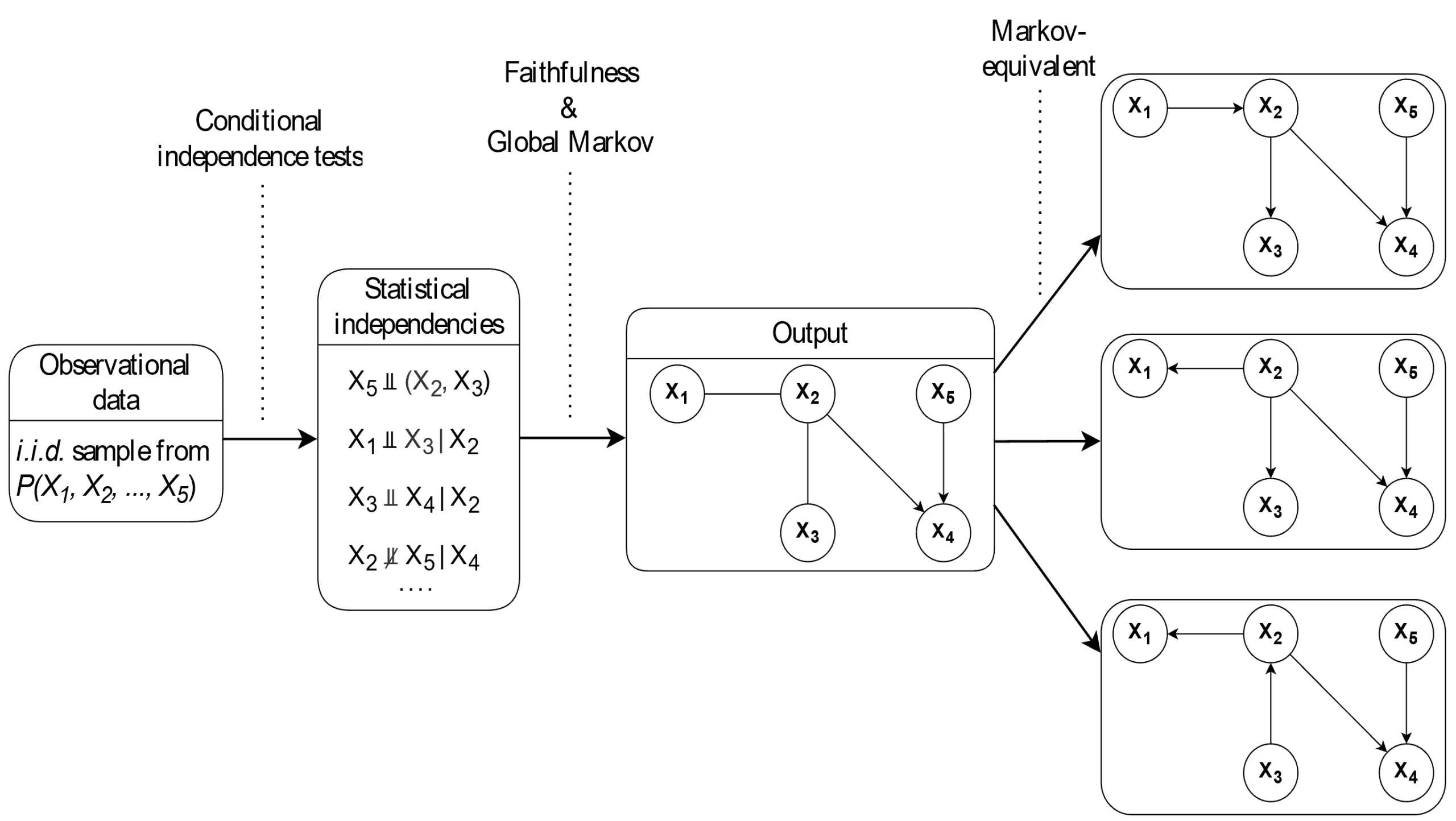
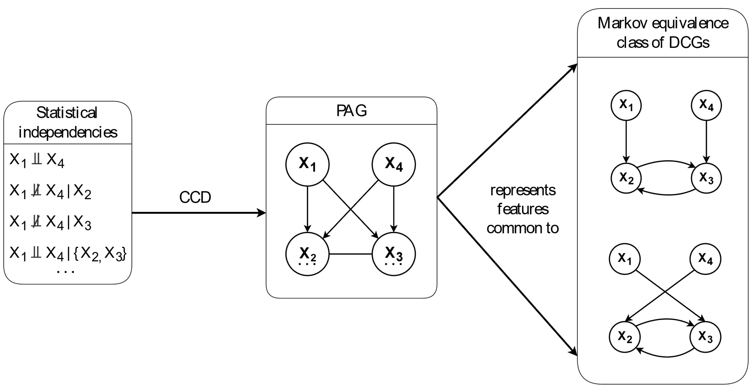
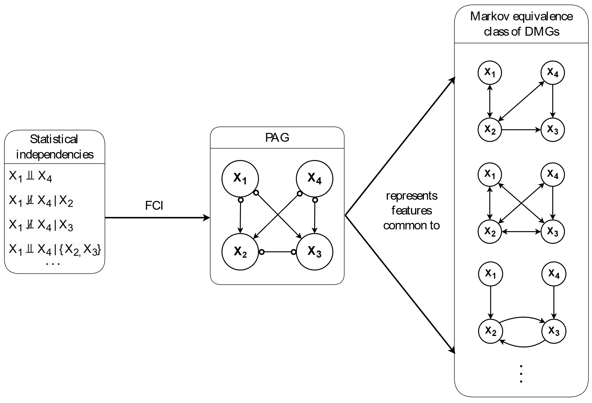
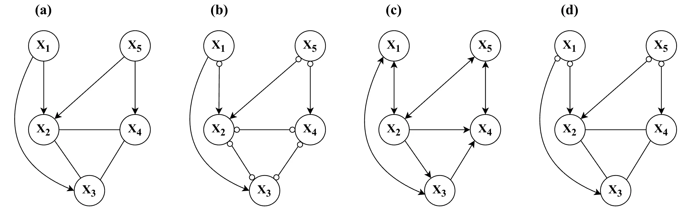
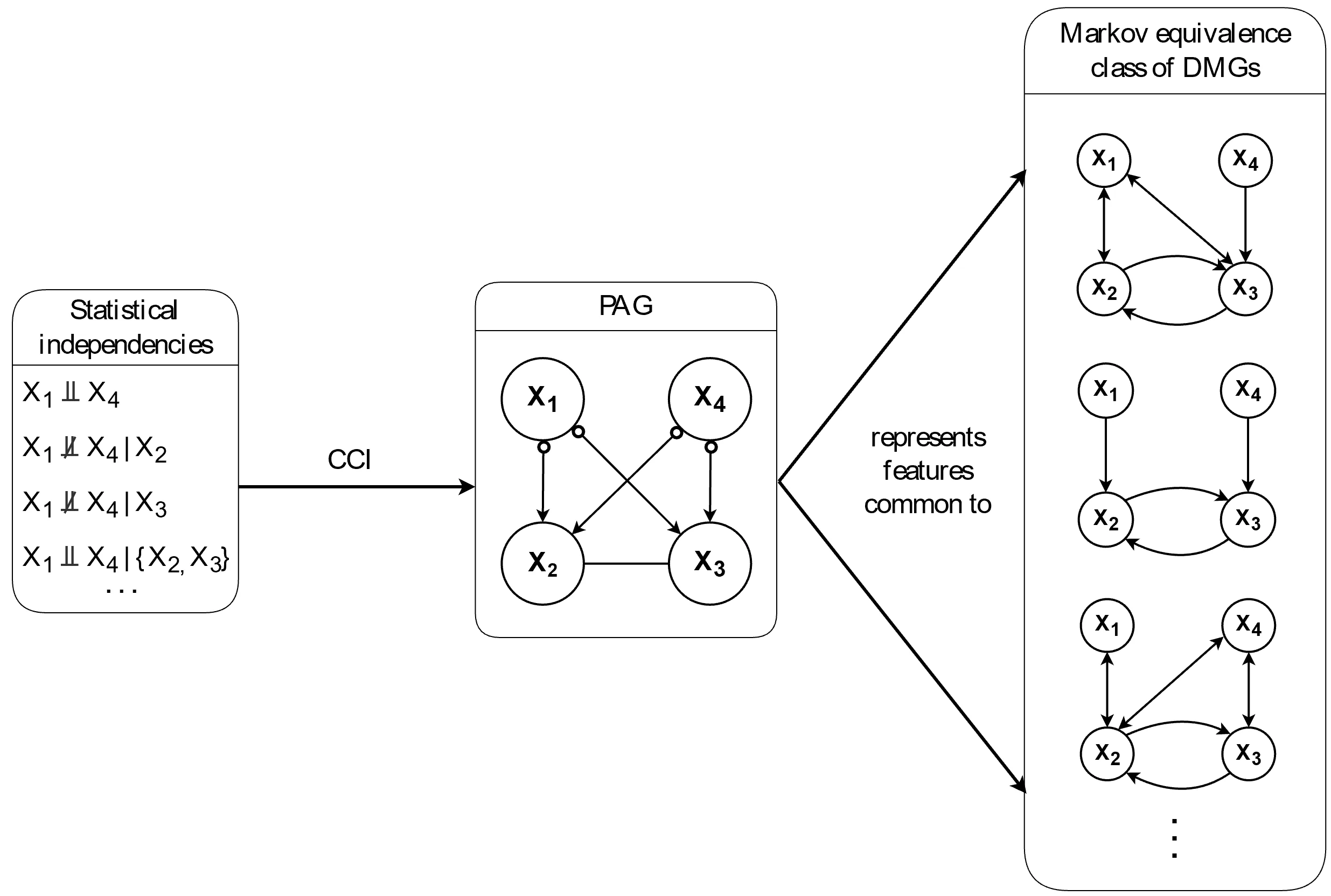
) in the graph. As a result, the Markov equivalence class tends to be relatively large.

CCI Algorithm

The CCI algorithm combines features of both the CCD and FCI algorithms. It can identify cyclic causal structures, similar to CCD, and can handle latent confounding, similar to FCI (Strobl, 2019). Employing a combined approach, however, comes at a cost; the algorithm requires more complex edge-endpoint inferences and lengthy orientation rules. For a detailed explanation of each step of the CCI algorithm, see Appendix C in the SOM.

CCI Output Representation: Partial Ancestral Graph (PAG)

As with the other two algorithms, CCI generates a PAG that captures the common ancestral relationships among equivalent graphs. To account for the presence of latent confounding in the infinite causal graph space, as described in Section 3.3.1, CCI also uses bidirected edges (↔). Apart from that, the interpretation of the other types of edges in PAGs estimated by CCI is the same as that described in Section 3.2.1 for the CCD output. In the following section, we will briefly outline the steps of CCI with the same example DCG (from Figure 1(b)) that has been used throughout the paper and examine the interpretation of the resulting PAG.

Steps of CCI Algorithm

The CCI algorithm consists of seven steps in total, the first two of which are identical to those of the other algorithms (i.e., skeleton discovery and collider structure orientation), and the remaining steps are similar to the further orientation rules implemented in CCD and FCI. Same as the others, CCI initiates with a PAG that is fully connected with ⧟ edges between every pair of variables (Figure 8(a)). After running the skeleton discovery procedure (i.e., step 1), the ancestral skeleton is estimated, as shown in Figure 8(b). Upon orienting the edges based on identified colliders (i.e., step 2), CCI produces the output shown in Figure 8(c). In the following orientation step (i.e., step 5), the edge between X2 and X3 is oriented utilizing Supsets — similar to step 4 of the CCD algorithm — which results in Figure 8(d). Since no additional edges are oriented in the subsequent steps, Figure 8(d) remains the final PAG. From this PAG, we can read off the following:

  1. X2 and X3 are not ancestors of X1 and X4 in every graph in Equiv(\(\mathcal{G}\)).
  2. X2 is an ancestor of X3 and X3 is an ancestor of X2 in every graph in Equiv(\(\mathcal{G}\)), implying a cyclic relationship between them.

Similar to FCI, the PAG obtained from CCI has more circle endpoints compared to the one obtained from CCD, due to its consideration of latent confounding. Figure 9 summarizes the operation of CCI, which is similar to that of FCI shown in Figure 7, with a relatively large Markov equivalence class of graphs. However, unlike the PAG from FCI where cycles are implied by the fully-connected edge with circle endpoints (⧟), the PAG from CCI clearly indicates a cyclic relationship between X2 and X3 with an undirected edge (—), which implies the reciprocal ancestral relationship between the two variables.

Figure 8

Trace of CCI algorithm.

Trace of the cyclic causal inference (CCI) algorithm showing steps in causality analysis.
Note. (a) depicts the fully-connected PAG, which is the starting point of the algorithm. (b) depicts the ancestral skeleton estimated in the same way as the CCD and FCI algorithms. (c) depicts the state of the PAG after orienting the collider structures in step 2. (d) depicts the state of the PAG after applying the extra orientation rules in step 5. No further orientation takes place in the subsequent steps, leaving (d) as the final PAG.

Figure 9

Summary of CCI algorithm operation.

Flowchart summarizing the operation of the CCI algorithm in network causal models.
Note. CCI constructs a partial ancestral graph (PAG) based on the observed statistical independencies, which captures the ancestral features common to every directed mixed graph (DMG) in a Markov equivalence class. Similar to the FCI algorithm, CCI accounts for the potential presence of latent confounding, which is represented by bidirected edges (), leading to more circle endpoints in the PAG. This generally results in a larger Markov equivalence class, as illustrated in the right-side of the figure.

Overview of Algorithms

Thus far, we have introduced three constraint-based causal discovery algorithms for cyclic graphs and discussed their characteristics. Based on our example (DCG from Figure 1(b)), the CCD algorithm may appear to be the preferred option, as it has less uncertainty in its output and correspondingly returns a smaller set of equivalent graphs. However, recall that the main advantage of the other two algorithms — FCI and CCI — is their ability to handle the presence of latent confounding, which commonly occurs in psychological research in practice (Rohrer, 2018).

The left-most panel of Figure 10 depicts the DCGs of two distinct data-generating processes: In the first, the causal graph consists of four variables X1, . . . , X4, while in the second, the causal graph consists of a fifth variable L1, which we will consider to represent a latent confounder. Now consider what output we would expect each of the algorithms reviewed above to return if they were fit to data generated from either of these data-generating systems: All three algorithms happen to generate the same PAG for these two different DCGs, shown in the remaining panels of Figure 10. Suppose the true underlying causal structure is the DCG without a latent confounder (top left in Figure 10). In that case, all three PAGs correctly depict the ancestral features of the true DCG. However, the PAG output by CCD is by far the most precise, as it contains no circle endpoints, thus representing the smallest equivalent set of graphs. Now, suppose the underlying causal structure is the DCG with a latent confounder (bottom left in Figure 10). Then, the PAG generated by CCD contains errors (i.e., X1 is not an ancestor of X2 and X3), while the PAGs estimated by FCI and CCI correctly represent the ancestral features of the true DCG. In the following section, we will conduct a simulation study to compare the performance of each algorithm under various conditions and investigate which algorithm is most suitable for situations likely to arise in psychological research.

Figure 10

Comparison of the partial ancestral graphs (PAGs).

Comparative diagram of partial ancestral graphs (PAGs) in different causal models.
Note. Two different DCGs are displayed in the first column, with subsequent columns showing the corresponding PAGs estimated by each algorithm. In this particular case, all three algorithms happen to produce identical PAG estimates for both DCGs.

Simulation

In this section, we present a simulation study to evaluate the performance of the three causal discovery algorithms introduced above under different conditions: namely, the sample size, number of variables in the graph, density, and presence of latent confounders. We investigate how these factors affect each algorithm’s performance and whether any algorithm outperforms the others in specific ways. In the following, we will first discuss the data generation process, simulation design, and evaluation metrics, before presenting the results of the simulation study.

Data Generation

We simulate data from the different cyclic models, as shown in Figure 11, all of which are characterized by linear relations and independent Gaussian error terms. These types of models are often used in psychological research, and for such cyclic models, the global Markov property — the necessary condition for constraint-based causal discovery — also holds, as discussed in Section 2.2.

To generate data, we first define a coefficient matrix B. A non-zero entry Bij indicates an edge from Xj to Xi with a strength of Bij. Thus, X1, …, Xp can be generated according to the following equation:

\(X_i = \sum_{r=1}^{p}B_{ir}X_r + \varepsilon_i,\)

for i = 1, …, p, where p is the number of vertices and ε are mutually independent N(0, 1) random variables. The variables X1,…,Xp then have a multivariate Gaussian distribution with a mean vector of zero and a covariance matrix Σ = (I B)−1(I B)T, where I denotes the identity matrix. Note that this data generation scheme is possible provided that (I B) is invertible, which is the case when the eigenvalues of B are smaller than one in absolute value, | λ | < 1 (Eberhardt et al., 2010). While this is guaranteed if B defines an acyclic model (Drton & Maathuis, 2017), for cyclic models, this does not always hold. To satisfy this condition, cyclic relations need to be not too strong so that the dynamical system converges to equilibrium (Rothenhäusler et al., 2015). We set fixed values for B to make the simulation results easier to track and interpret. When specifying the B matrices, we choose values within a range that is deemed reasonable (e.g., restricting the strength of cyclic relations to relatively small such that they do not diverge) and verify that the eigenvalues satisfy the equilibrium condition.[7] When this condition is violated, we adjust the parameters until it is satisfied. In addition, to ensure that the simulation results are not dependent on the specific values of the coefficient matrix B, we perform a sensitivity analysis. In this analysis, we randomly sample parameter values of B from a uniform distribution on [−0.9, −0.1] ∪ [0.1, 0.9] in each iteration. We then check whether the equilibrium condition is met, and if not, we re-sample the parameters until it is satisfied. In the following, we provide a detailed description of the simulation setup, which is replicated across both simulation studies.

Figure 11

Simulation settings.

Bar chart of simulation settings used to evaluate cyclic causality in psychological models.
Note. In our simulation study, we vary several factors such as the number of variables: p ∈ {5, 10}, the density: sparse / dense, the influence of a latent confounder: absence / presence, and the sample size: N ∈ {50, 150, 500, 1000, 2000, 3000, 4000, 5000, 7500, 10000}. This results in a 2 × 2 × 2 × 10
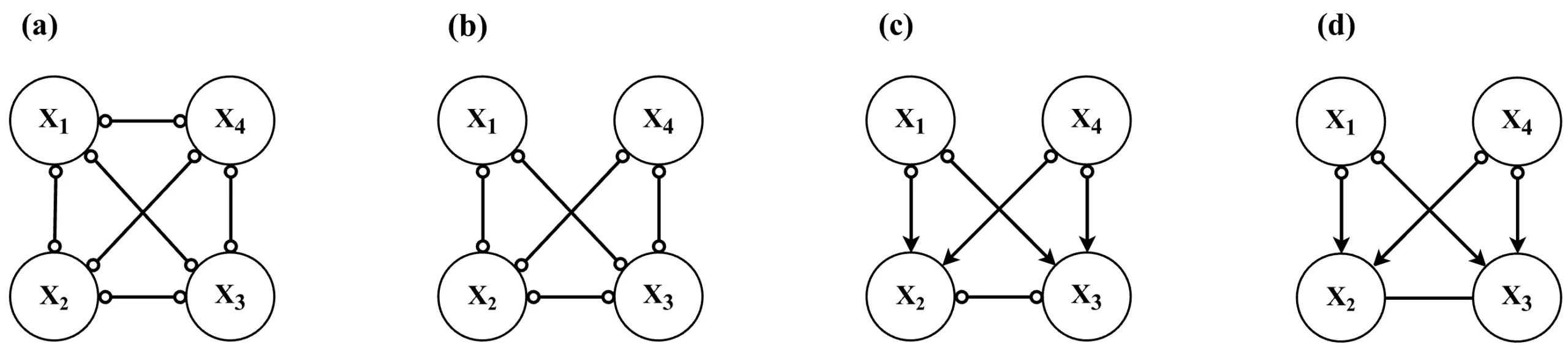
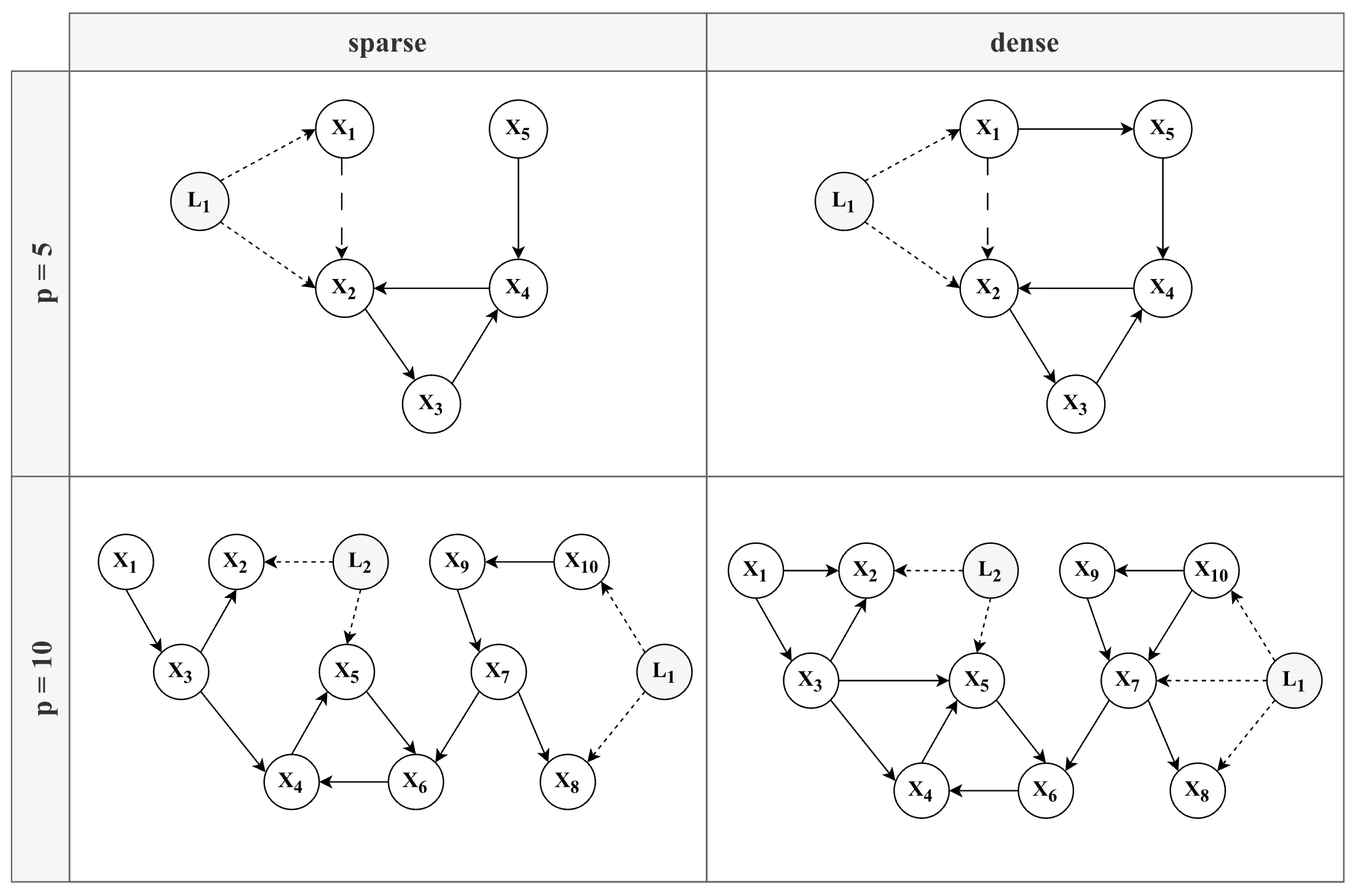
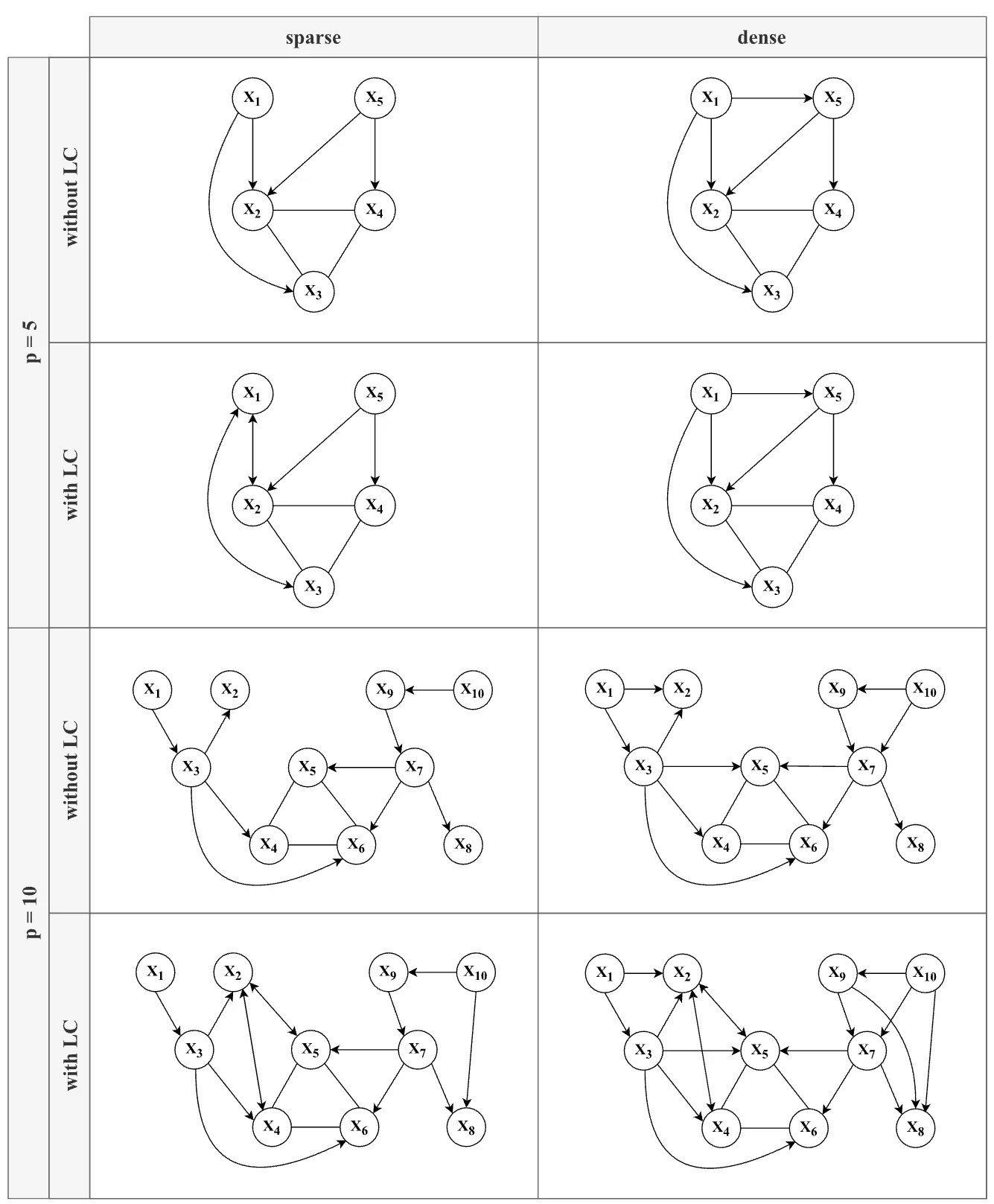
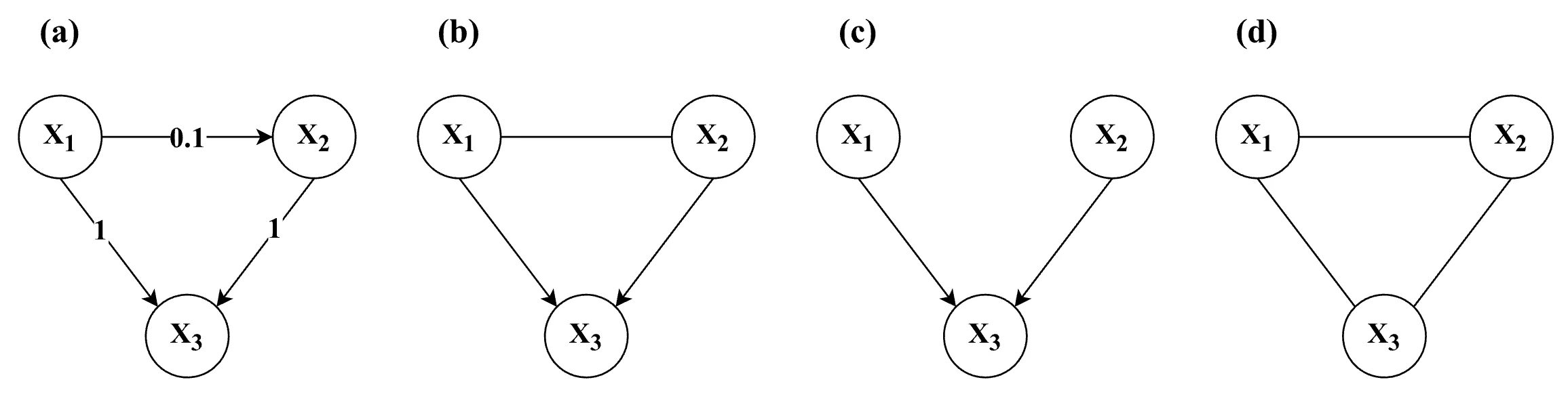
simulation design, with each combination of factors (except for N) yielding a unique model structure. Note that the edge between X1 and X2 (long-dashed line — —) in the 5-variable models (top row) is only present in the conditions without a latent confounder.

Simulation Setup

We test each algorithm under different conditions by varying the number of variables (rows in Figure 11) and the number of edges — the density (columns in Figure 11). We also explore the impact of unobserved confounding by introducing latent variables (L1 and L2 in Figure 11), as latent confounding is a common issue in psychological research, particularly when it comes to inferring causal relationships (Hallquist et al., 2021; Rohrer et al., 2022). Lastly, we vary the sample size ranging from small to moderately large, N ∈ {50, 150, 500, 1000, 2000, 3000, 4000, 5000, 7500, 10000}, for every simulated cyclic model. This leads to a 2 × 2 × 2 × 10 design; number of variables × density × latent confounder (presence/absence) × sample size. We simulate each condition 500 times, estimating three PAGs per iteration using each algorithm. See Figure 11 for an overview of the different types of cyclic models used in the simulation. These models precisely depict the ones utilized in the simulation.

To test for conditional independence, we employ partial correlations since the variables in our simulated data have linear relations with additive Gaussian errors. In such cases, conditional independence is equivalent to zero partial correlation (Lawrance, 1976). Throughout the study, we use a fixed alpha level of 0.01 (α = 0.01) for conducting the conditional independence tests, which is a commonly used value in causal discovery studies with moderate sample sizes (Malinsky & Danks, 2018). However, we acknowledge that following the fixed α convention is not straightforwardly justified (Strobl et al., 2017). To address this, we perform another sensitivity analysis where we adjust the α level based on the sample size. Further elaboration on this analysis will be provided in Appendix H in the SOM. All simulations are performed using R software version 4.2.3 (R Core Team, 2023).

Evaluation Metrics

As discussed in Section 3, the algorithms attempt to recover the ancestral graphs implied by the underlying DCG. In order to evaluate the performance of each algorithm, we compare how well it recovers the true ancestral graph. To do this, we first need to construct a true ancestral graph for each simulated condition, which can then be compared to the estimated graphs. The true ancestral graph for each DCG considered in our simulation study is shown in Figure 12. For those interested, a step-by-step procedure for deriving a true ancestral graph from a DCG is provided in Appendix E in the SOM.

For assessment, we use both local and global evaluation metrics. At the local level, we look at the individual edge-endpoints and compare whether they match the corresponding endpoint of the true graph. At the global level, we look at the graph structure as a whole and measure the distance between the true and estimated graph, assessing how closely the estimated graph’s structure matches the true graph’s structure. As the local metrics, we utilize precision, recall, and uncertainty rate.

\( \begin{align*}
\text{Precision} &= \scriptstyle \frac{\text{True Positive}}{\text{True Positive } + \text{ False Positive}} \\
\text{Recall} &= \scriptstyle \frac{\text{True Positive}}{\text{True Positive } + \text{ False Negative}} \\
\text{Uncertainty rate} &= \scriptstyle \frac{\text{Number of circle endpoints } (\circ)}{\text{Total number of edge-endpoints}}
\end{align*}
\)

Precision reflects the prediction accuracy (i.e., out of all predicted cases, how many are correct), and recall reflects the retrieval rate (i.e., out of all true cases, how many are retrieved). Each edge-endpoint in a resulting graph can fall into one of four categories: no edge-endpoint (null), arrow head (>), arrow tail (−), and circle (○). Given that circle endpoints indicate that an algorithm is unsure of the direction of causal relations, the uncertainty rate is defined as the proportion of the circle endpoints present in the output. For example, consider the example PAG shown in Figure 13(b). The uncertainty rate for this PAG can be calculated as \(\frac{3}{20}\), where the number of circle endpoints is 3, and the total number of edge-endpoints is 20 (\(\binom{5}{2} \times 2 = 20\)). For the other non-circle endpoints, we compute the precision and recall. As an example, suppose that Figure 13(a) is the true ancestral graph and Figure 13(b) is the estimated PAG output. We can then construct a confusion matrix of the estimated versus true edge-endpoints.[8] Based on the confusion matrix shown in Figure 13(c), we can compute the precision and recall for each type of non-circle endpoints. For the arrow head (>), for instance, the precision and recall are computed as: precision = \(\frac{4}{4 + 3 + 0}\) and  recall  = \(\frac{4}{4 + 0 + 0}\). Note that the circle endpoints are not considered in the calculation of precision and recall and therefore they are greyed out in the confusion matrix.

As the global metric, we use the structural Hamming distance (SHD) (de Jongh & Druzdzel, 2009). SHD quantifies the level of differences between two graphs by counting the number of edge insertions, deletions, and direction changes required to move from one graph (estimated graph \(\hat{\mathcal{G}}\)) to the other (true graph \(\mathcal{G}\)). It can be formulated as: SHD = A + D + C, where A, D, and C represent the number of added edges, deleted edges, and changes in edge-endpoints, respectively. A lower SHD value suggests that the estimated graph (\(\hat{\mathcal{G}}\)) is more closely aligned with the true graph (\(\mathcal{G}\)), indicating a better recovery of the true graph structure. For example, the SHD value for the PAG output in Figure 13(b) — provided that the true ancestral graph is Figure 13(a) — is 6, which is calculated by summing: 0 (A) + 0 (D) + 6 (C). As such, in contrast to the precision and recall metrics, which omit circle endpoints in their computation, and the uncertainty metric, which directly counts only the degree of circle endpoints, the SHD metric treats circle endpoints as equivalent to any other type of endpoint error.

Figure 12

True ancestral graph for each condition.

Graph of the true ancestral graph for each condition in psychological causal research.
Note. Each panel in the figure depicts the true ancestral graph for each simulated condition. Directed edges denote ancestral relationships (A  B means A is an ancestor of B), bidirected edges indicate the presence of latent confounders (A  B means there is a latent confounder between A and B), and undirected edges denote mutual ancestral relationships, thereby indicating cyclic relationships between the corresponding variables (A B means A and B are ancestors of each other, implying the presence of a cyclic relationship between them). For more information on how to derive the true ancestral graph from a DCG, see Appendix E in the SOM. p = number of variables; LC = latent confounder.

Figure 13

Example performance evaluation.

Bar chart illustrating example performance evaluation in cyclic causal discovery.
Note. For the purpose of illustration, we consider the 5-variable sparse condition with a latent confounder shown in the top left panel of Figure 11. Panel (a) displays the true ancestral graph, while panel (b) presents an example of the estimated PAG output. Panel (c) shows the confusion matrix for the estimated versus true edge-endpoint, where the true endpoints are presented in rows and the estimated endpoints in columns. There are in total four possible edge-endpoints that can occur in an output: arrowhead (>), arrow tail (—), null (no endpoint), and circle (○). The circle endpoints, however, are not counted toward the calculation of precision and recall, and thus are greyed out in the table.

Simulation Results

In this section, we will report the results of the simulation study using the fixed values of B matrices. First, we will present the overall performance of the considered algorithms based on the structural Hamming distance (SHD), and then we will take a more detailed look into their performance using precision, recall, and uncertainty rate.

Performance on Global Metric

The SHD values for each algorithm per condition are shown in Figure 14, where the points and shaded area represent the average SHD values of 500 iterations and the corresponding interquartile range (IQR), respectively. As discussed in Section 4.3, a lower SHD value indicates a better performance, as it means that the estimated graph is closer to the true graph. Overall, the FCI and CCI algorithms perform better in sparse conditions, while the CCD algorithm outperforms the others in dense conditions. Additionally, the performance of all three algorithms is generally worse in dense conditions than in sparse conditions. Interestingly, in small models (p = 5) with high density (second and fourth columns from the top row of Figure 14), the SHD values momentarily decrease and then start increasing again as the sample size (N) becomes larger. This is partly against our expectation that the SHD values would decrease monotonically with increasing sample size. Furthermore, we do not observe any significant contrasting patterns between conditions with and without latent confounders. This is contrary to our expectation that CCD would perform relatively better in conditions without latent confounders, while FCI and CCI would perform better in conditions involving latent confounders as they can handle latent confounding.

Figure 14

Structural Hamming distance (SHD).

Line graph showing Structural Hamming distance (SHD) across causal models.
Note. The sample size (N) is shown on the x-axis, and the SHD values are shown on the y-axis. Each point represents the average SHD value across 500 simulations, while the shaded area represents the interquartile range (IQR). p = number of variables; LC = latent confounder.

Performance on Local Metrics

In what follows, we will further examine the performance of the algorithms using local metrics, while addressing some of the unexpected findings discussed previously in Section 4.4.1. These include (i) the observation that CCI and FCI outperform CCD in sparse conditions, even when latent confounders are not present and (ii) the SHD values increase instead of decreasing with increasing sample size in the 5-variable dense conditions.

The results for precision, recall, and uncertainty rate for each algorithm are summarized in Figure 15, where each point represents the average value of the metrics over 500 iterations in the corresponding condition, and the shaded area represents the interquartile range (IQR) of the values obtained. As with the SHD results, we observe that the CCI algorithm generally exhibits high precision and recall in sparse conditions. On the other hand, the FCI algorithm records low precision and recall, even lower than CCD. This might seem contradictory at first glance, given that FCI has better SHD values than CCD in most conditions (except for a few dense cases). However, this can be explained by the overall low uncertainty rate of FCI as opposed to the high uncertainty rate of CCD, as shown in Figure 15(c). FCI tends to guess directions without necessarily outputting circles, while CCD tends to produce circles rather than guessing directions. This contrasting behavior consequently leads to FCI having better SHD values than CCD. To illustrate this point further, we examine the most frequently estimated PAGs from each algorithm in the 5-variable sparse condition without a latent confounder presented in Figure 16.[9] In Figure 16(c), we can observe the typical orienting behavior of FCI, where it guesses the directions for every edge endpoint (i.e., not conservative), in contrast to CCD, which often produces circles (i.e., conservative), as shown in Figure 16(b). Based on the true graph shown in Figure 16(a), we can calculate the SHD: 9 for CCD (Figure 16(b)), 7 for FCI (Figure 16(c)), and 4 for CCI (Figure 16(d)). As such, FCI achieves a lower SHD value than CCD, despite having relatively lower precision and recall values due to some incorrectly predicted edge-endpoints.[10] This highlights the distinct properties of the metrics used in our study. SHD is agnostic about whether an algorithm is conservative or less conservative, since it measures all differences between the estimated and true graphs, including the circle marks. As a result, it penalizes an algorithm for being conservative as much as for making incorrect predictions. On the other hand, precision and recall only consider non-circle endpoints, while disregarding the circle marks. Therefore, they penalize an algorithm for making incorrect predictions but not for being conservative (i.e., producing circles).

Figure 15

Precision, recall, and uncertainty rate.

Bar graph depicting precision, recall, and uncertainty rate in causality analysis.
Note. The sample size (N) is shown on the x-axis, and the corresponding metric values are shown on the y-axis. Each point on the graph represents the average of iteration-specific values of precision (top panel), recall (middle panel), and uncertainty rate (bottom panel) for each condition, with the shaded area indicating the interquartile range (IQR). p = number of variables; LC = latent confounder.

In addition, the comparison between CCI and CCD based on precision and recall in Figure 15 reveals only a subtle difference in performance, even in the 5-variable sparse conditions where CCI outperformed CCD significantly in terms of SHD. This can be again attributed to CCD having a comparatively high uncertainty rate. From the PAG estimated by CCD in Figure 16(b), it can be observed that all of the directions predicted by CCD are correct, but the PAG contains a fairly large number of circle endpoints. These circle endpoints lead to a poorer SHD value for CCD, even though it exhibits comparably high precision and recall for correctly predicting directions. Moreover, further examination of the resulting PAGs shows that CCI performs better than CCD in detecting mutual ancestral relationships in cyclic structures. For instance, in Figure 16(b), CCD assigned all circle marks to the cycle involving X2, X3, and X4, while CCI correctly identified the mutual ancestral relationships in the cycle with undirected edges (—), as shown in Figure 16(d). This superiority of CCI in recovering mutual ancestry in cycles was consistently observed in other conditions as well, suggesting that this property is a significant factor contributing to CCI’s overall better performance compared to other algorithms, even in the absence of latent confounding.

Figure 16

Frequently estimated PAGs in the 5-variable sparse condition without a latent confounder.

Visualization of frequently estimated partial ancestral graphs in sparse network conditions.
Note. Panel (a) shows the true ancestral graph of the 5-variable sparse condition without a latent confounder. Panels (b), (c), and (d) present the most frequently occurring PAGs in the 5-variable sparse condition without a latent confounder resulted from the CCD, FCI, and CCI algorithms, respectively. They were obtained by picking the most frequent type of edge-endpoints produced by each algorithm from 500 simulations with a sample size of 1000.

With respect to the unexpected increase in SHD values in the 5-variable dense conditions, we also observe an unusual decrease in precision and recall as the sample size increases (second and fourth panels from the top rows of Figure 15(a) and Figure 15(b)), along with an increase in the uncertainty rate (second and fourth panels from the top row of Figure 15(c)), indicating that more circle endpoints appear in the resulting PAGs as the sample size grows. Learning a dense causal structure is generally more challenging, because there is less information available about the conditional independence relations when a large number of vertices are connected by edges (i.e., almost everything is dependent on everything else). This problem is further compounded in the presence of cycles, as all variables that are part of cycles are completely dependent on each other, making it even more challenging to obtain information about independence relations. Therefore, algorithms tend to fail to orient any edges and mostly output only circle endpoints in dense cyclic graphs. The decline in precision and recall, along with the rapid increase in uncertainty rate observed in Figure 15 for the 5-variable dense conditions, are primarily due to this challenge in high-density situations — as the sample size becomes larger, relatively weak edges start getting picked up by the algorithms, leading to denser structures that make causal discovery exceedingly difficult.

However, interestingly, we also note a slight increase in both precision and recall for the 5-variable dense conditions when the sample size is relatively small, accompanied by a small drop in the SHD (second and fourth panels from the top row of Figure 14). This might seem counterintuitive, as we typically expect the algorithms to learn causal structures more accurately with larger sample sizes. But, in fact, it is possible to lose the correct edge orientation when the sample size is large, particularly in the case of a dense graph with weak edges (Eigenmann et al., 2017). Figure 17 illustrates a simple example case where the inclusion of a weak edge leads to the loss of edge orientation. With a large sample size, algorithms are likely to pick the weak edge between X1 and X2, resulting in an uninformative undirected graph, as shown in Figure 17(d). However, with a small sample size, algorithms are more likely to miss the weak edge and identify the collider X3, thereby obtaining the correct edge orientation, as shown in Figure 17(c). In our 5-variable dense scenarios, we run into a similar situation. There is a relatively weak edge between X2 and X5, which is not detected by algorithms when the sample size is small, resulting in some correctly oriented edges. However, as the sample size becomes larger, the weak edge gets detected, and the algorithms fail to orient any edges, thus yielding completely undirected graphs (see Appendix F in the SOM for a more detailed explanation of the results in our 5-variable dense cases). This explains the small dips at the beginning of the SHD line graphs (Figure 14) and brief spikes in the precision and recall graphs (Figure 15) for the 5-variable dense conditions with relatively small sample sizes.

Figure 17

An example dense graph with a weak edge.

Example of a dense psychometric network graph with a weak causal edge highlighted.
Note. Panel (a) shows the true graph. Panel (b) displays the desired output where the collider structure is correctly oriented while the weak edge between X1 and X2 is also identified. Panel (c) presents the output graph when an algorithm fails to detect the weak edge between X1 and X2 but correctly orients the collider structure. Panel (d) displays the output graph when an algorithm detects the weak edge between X1 and X2. This results in a denser graph with less information on independencies, leading to the loss of orientation of the collider structure.

To summarize, both CCD and CCI algorithms show good performance, with CCI slightly outperforming in sparse conditions and CCD in dense conditions. However, CCD tends to be more conservative in terms of edge orientation and produces more circle endpoints than CCI, which often results in higher SHD values. In contrast, FCI demonstrates poor performance across most conditions, which is not immediately obvious when considering only the global metric, SHD. Further analysis of local metrics reveals that FCI often makes quick directional inferences without producing circle marks, resulting in comparably good SHD values but low precision and recall values.

In addition, to investigate the robustness of our findings against the specific parameter values chosen in this simulation, including the coefficients of B matrices and the value of α, we conducted additional simulations as part of sensitivity analyses. In one of these simulations, we randomly sampled parameter values for B at each iteration. Our results were similar to the original simulation, with a few minor differences; we do not find any unusual kinks or dips in the performance curves with small sample sizes in the 5-variable dense conditions (see Figure 18). Instead, we find that the algorithms’ performance steadily improves with increasing sample size, which aligns with our initial expectation. In another simulation, we varied the  level according to the sample size; decreasing  as the sample size (N) increased such that αN 0 as N → ∞ at a suitable rate.[11] It is commonly suggested to adjust α according to the sample size in order to ensure consistent results of conditional independence tests (Mooij et al., 2020; Colombo et al., 2012).[12] Overall, the results show no significant differences in the observed patterns across all conditions, indicating that the effect of adjusting α is negligible. The detailed results of these sensitivity analyses can be found in Appendix G and Appendix H in the SOM, respectively.

Figure 18

Performance in the 5-variable dense condition without a latent confounder.

Bar chart showing performance metrics in the 5-variable dense condition without latent confounders.
Note. This figure illustrates the performance of each algorithm in the 5-variable dense condition without a latent confounder, where the coefficients of B were randomly sampled. The sample size (N) is shown on the x-axis, and the corresponding metric values are shown on the y-axis. Each point represents the mean value of each metric across 500 simulations, and the shaded area represents the interquartile range (IQR). Note that the performance under the 5-variable dense condition with a latent confounder shows more or less the same patterns (see Appendix G in the SOM for details).

Empirical Example

In this section, we present an empirical example where we apply the three causal discovery algorithms studied above to real psychological data to assess their practical applicability. We begin by introducing the dataset and then present the output of each algorithm, along with the corresponding statistical network model. Our goal is to assess whether the output PAGs carry meaningful information about the causal structure and to compare the insights gained from these PAGs with those obtained from the statistical network model. To aid researchers with applying these methods in their own research, we provide an annotated script to reproduce our empirical analysis in the reproducibility archive of this paper: https://github.com/KyuriP/Discovering CCM/tree/main/empirical example.

Table 2
Summary of depression symptoms.
 
Symptom (abbreviation)Mean (SD)
1. Sleep-onset insomnia (ons)1.20 (1.07)
2. Middle insomnia (mdd)1.44 (1.07)
3. Early morning awakening (lat)0.81 (1.07)
4. Hypersomnia (hyp)1.01 (0.99)
5. Sadness (sad)1.55 (0.94)
6. Decreased appetite (dcp)0.49 (0.72)
7. Increased appetite (inc)0.44 (0.87)
8. Weight loss (wghtl)0.50 (0.94)
9. Weight gain (wghtg)0.67 (1.04)
10. Concentration impairment (cnc)1.48 (0.87)
11. Guilt and self-blame (glt)1.56 (1.17)
12. Suicidal thoughts (scd)0.63 (0.82)
13. Anhedonia (anh)1.27 (1.05)
14. Fatigue (ftg)1.33 (0.95)
15. Psychomotor retardation (rtr)0.66 (0.81)
16. Agitation (agt)1.10 (0.93)
Note. SD = Standard Deviation.

Data and Model Fitting

The dataset used in our empirical example is from McNally et al. (2017), where the authors focused on examining the causal relationships between symptoms of obsessive-compulsive disorder (OCD) and depression.[13] Notably, the authors expressed a particular interest in investigating cyclic causal relationships. However, the causal discovery methods they were familiar with were only applicable to acyclic causal structures, leading them to use a statistical network model. Although they acknowledged that the network captures statistical rather than causal relationships, they argued that statistical network analysis addresses a key limitation of the acyclic causal discovery algorithm, which is excluding the possibility of feedback loops (cycles). Their explicit interest in cyclic causal discovery makes this dataset an ideal candidate for testing the cyclic causal discovery algorithms discussed in the current paper.

The dataset consists of 408 observations and 26 variables, comprising 16 depression symptoms and 10 OCD symptoms, all with no missing values. The severity of each symptom was measured using a four-point Likert scale, with 0 indicating no symptoms and 3 indicating extreme symptoms. The participants’ age ranged from 18 to 69 years, with a mean of 31.1 and a standard deviation of 12.2. In this paper, we focus our analysis on a subset of the variables — depression symptoms — in order to keep the model size manageable and facilitate the interpretation of the estimated PAGs. For a summary of the depression symptom variables, please refer to Table 2.

To compare the results of the cyclic causal discovery algorithms with those of network analysis, we estimated a Gaussian graphical model (GGM). In a GGM, the edges signify partial correlations between pairs of nodes, controlling for the rest of nodes in the network with the assumption that the variables follow a normal distribution. (Epskamp et al., 2018b). To obtain a sparse network, we used the graphical lasso (glasso) method to regularize partial correlations, such that small partial correlations are driven to zero and therefore do not appear in the network (Friedman et al., 2008). For the causal models, we ran all three algorithms (CCD, FCI, and CCI) while setting the alpha level to 0.01 (α = 0.01) as a rough way to correct for spurious edges resulting from a relatively large set of variables (Zhang et al., 2012). As in the simulation study, we used partial correlations to test for conditional independencies. In the following section, we will present the estimated models and interpret the findings from each model while comparing them to one another.

Empirical Analysis Results

The causal models estimated by each algorithm (i.e., PAGs) and the GGM are depicted in Figure 19. Upon examining the GGM presented in Figure 19(a), we can identify three symptom clusters that are highly interconnected within themselves but less connected with the rest. On the right-hand side of the network, we see symptoms related to physical weight and appetite: weight gain (wghtg), weight loss (wghtl), increased appetite (inc), and decreased appetite (dcp), with particularly strong partial correlations between inc wghtg and dcp wghtl. Towards the bottom of the network, we see three symptoms relating to insomnia: early morning awakening (late), sleep onset insomnia (ons), and middle insomnia (mdd). The remaining items towards the left side of the network form a single cluster. Here, we observe strong connections among several symptoms, including psychomotor retardation (rtr) – concentration impairment (cnc) – fatigue (ftg) – anhedonia (anh) – sadness (sad) – suicidal thoughts (scd). Especially, fatigue, anhedonia, and sadness emerge as the most central symptoms based on the number and strength of connections they have with the other nodes in the network. As McNally et al. (2017) note, this is in accordance with the general clinical observations where sadness and anhedonia, as the two gateway symptoms, are necessary for a diagnosis of depression.

Figure 19

A statistical network model and PAGs estimated from empirical data.

Comparative visual of a statistical network model and estimated partial ancestral graphs from empirical data.
Note. Panel (a) shows the statistical network model (i.e., Gaussian graphical model) estimated from the empirical data on depression symptoms. Panels (b), (c), and (d) show the PAG estimated by the CCD, CCI, and FCI algorithm, respectively. ons = sleep onset insomnia; mdd = middle insomnia; lat = late (early morning awakening); hyp = hypersomnia; sad = sad; dcp = decreased appetite; inc = increased appetite; wghtl = weight loss; wghtg = weight gain; cnc = concentration impairment; glt = guilt; scd = suicidal thoughts; anh = anhedonia; ftg = fatigue; rtr = psychomotor retardation; agt = agitation.

Looking at the PAG from the CCD algorithm shown in Figure 19(b), we can read off information about possible directions of causal relations between these variables. Overall, the estimated structure is not too different from that of the GGM, in terms of the presence or absence of edges, but it is more sparse. The estimated PAG from CCD reveals that fatigue and anhedonia still remain central nodes. However, in the causal graph, we can now attribute their centrality to the fact that fatigue is the (indirect) effect of many variables, and anhedonia is the (indirect) cause of many variables — the directional information that could not be obtained from the statistical network model above. The three-cluster structure observed in the GGM is also present in this PAG, with only a few edges linking the separate clusters. For example, on the right side of the graph, we can see that increased appetite (inc) is an ancestor of guilt (glt), and weight loss (wghtl) is an ancestor of early morning awakening (lat). Anhedonia (anh) also plays an important role in linking these separate symptom clusters, acting as an ancestor of both early morning waking (lat) and decreased appetite (dcp). On the left side of the graph, we observe an intricate network where most of the variables are involved in a web of cyclic ancestral relationships.[14] While it is tempting to interpret these ancestral patterns as those of direct cyclic causal relationships, readers should exercise caution. As previously demonstrated in Figure 4 from Section 3.2.1, cyclic causal relationships would be represented by undirected edges (—) in a PAG, not by patterns of directed ancestral relationships. In addition, the dotted-underlining of the variables such as fatigue ( ftg ) and guilt ( glt ) likely indicates that not all the ancestral relationships shown in this PAG can be mapped onto direct causal relationships in the corresponding DCG. Hence, the structures that appear as cycles in this PAG may not necessarily imply the same direct causal cycles in the underlying DCG. Despite the rather complicated nature of interpreting the PAG, we believe that it provides more insightful information on the causal dynamics of depression symptoms when compared to the GGM, given that the PAG provides directional information, indicating the causal flow of variables, which cannot be obtained from the GGM.

As we have outlined previously, a key limitation of the CCD algorithm is its reliance on the assumption of causal sufficiency (i.e., the absence of unobserved confounders). If this assumption is violated, the PAG will not accurately reflect the causal relationships. This limitation is addressed by the CCI and FCI algorithms, which allow for the presence of latent confounders. Figure 19(c) and Figure 19(d) show the estimated PAGs from CCI and FCI, respectively. The overall structure is reminiscent of the PAG obtained from CCD, with three distinct clusters. However, the PAGs generated by CCI and FCI contain fewer edges, resulting in more independent clusters. Also, these PAGs feature bidirected edges (↔), indicating the presence of latent confounders. The CCI algorithm, in particular, produced a significant number of bidirected edges, suggesting the presence of latent confounders between almost every variable (see Figure 19(c)). On the other hand, the PAG generated by FCI shown in Figure 19(d) has only a few bidirected edges but more circle endpoints. Both CCI and FCI identified some common bidirected edges, including cnc ftg, agt cnc, and agt glt, indicating that there are likely to be latent confounders present between these variables. This is consistent with previous research that has shown, for example, chronic physical illness to be a potential contributing factor to symptoms such as concentration impairment (cnc) and fatigue (ftg) (Menzies et al., 2021;  Goërtz et al., 2021; de Ridder et al., 2008). In addition, both CCD and FCI predicted some common directional features, such as rtr \(\ast\mkern-8mu\rightarrow\) ftg, hyp \(\ast\mkern-8mu\rightarrow\) ftg, scd \(\ast\mkern-8mu\rightarrow\) glt, and anh \(\ast\mkern-8mu\rightarrow\) dcp. For example, anh \(\ast\mkern-8mu\rightarrow\) dcp means that anhedonia may or may not cause decreased appetite, but decreased appetite does not cause anhedonia, which also partly aligns with a previous study, where appetite loss is identified as one of the features of anhedonia (Coccurello, 2019).

Overall, this example highlights that the PAGs produced by cyclic causal discovery algorithms provide unique insights into possible causal relationships that cannot be gained through network analysis alone. For instance, interpreting the CCD output (Figure 19(b)) provides some directions for investigating potential intervention targets, a type of inference often of interest in psychological network analysis (Ryan et al., 2022; Ryan & Hamaker, 2022; Rodebaugh et al., 2018; Bringmann et al., 2019). Anhedonia (anh) could be a promising intervention target as it (indirectly) causes many other symptoms and acts as a bridge that connects different clusters of symptoms. Guilt (glt) also acts as a bridge to many sub-clusters of symptoms, and so might be effective in breaking ties and deactivating the overall system. These causal inferences are challenging to make in network analysis, which lacks directionality, making it difficult to determine the driving node. By solely looking at Figure 19(a), one might assume that fatigue should be the target node due to its numerous thick edges, but in the causal structure, this may not be accurate as it is primarily an effect node without direct causal influence on other symptoms. In addition, our findings show that the algorithms generally agree on many features, including the presence or absence of causal relations and some of the causal directions, which are in line with prior research, further enhancing their plausibility. However, the choice of which output PAG to pay most attention to depends on our degree of confidence in the assumptions underlying each algorithm. While the most informative PAG is generated by CCD, it makes strong assumptions about the absence of unobserved confounding and the linearity of causal relations. On the other hand, CCI suggests that most or all relationships between symptoms are likely influenced by latent confounding. FCI also flags the possibility of latent confounding but recovers different directed ancestral relations than CCI, as it makes use of different orientation rules. In general, FCI may be preferred over CCI when the linearity assumption does not hold, but CCI may be more appropriate in cases where the linearity assumption holds, as suggested by our simulation study.

Finally, to ensure the reliability of our findings, we conducted an additional stability analysis by running the algorithms on multiple random subsets of the data and retaining only the causal relations that were consistently discovered. This analysis confirmed that the identified causal relations from our original analysis are reliable such that they are not undermined by small variations in the data. Further details regarding this analysis can be found in Appendix I in the SOM.

Discussion

In this paper, we studied constraint-based cyclic causal discovery algorithms in typical psychological research settings, with a focus on identifying an effective algorithm for studying the underlying cyclic causal structure. We provided a comprehensive overview and didactic treatment of cyclic causal discovery by outlining the properties of three specific algorithms: CCD, FCI, and CCI. We assessed the performance of these algorithms under varying conditions through a simulation study, and we also demonstrated their practical applicability in psychological research by applying them to empirical data. Our results suggested that the CCI algorithm generally performed well, particularly in sparse conditions, and the CCD algorithm tended to outperform the others in dense conditions. The FCI algorithm performed poorly across all conditions, mostly guessing the directions of edges, though notably, our simulation was limited to studying systems with linear causal relations. Our empirical example showed that causal discovery methods provided more detailed and richer insights into the underlying causal dynamics of depression than the statistical network model, which in fact was found to contain numerous spurious edges, rendering it unsuitable for serving as a causal skeleton (Ryan et al., 2022).

With this paper, we aimed to provide empirical researchers with guidance on selecting an appropriate cyclic causal discovery algorithm for studying causal relationships. Our findings indicate that no single algorithm is suitable for all cases, and the choice of algorithm should be based on the characteristics of the causal system of interest. If the causal system is believed to be relatively sparse, then the CCI algorithm may be preferred, as it performs well under such conditions. Conversely, if the system is considered to be comparatively dense, researchers may opt for the CCD algorithm. Also, researchers need to consider their priorities when selecting an algorithm. If avoiding incorrect edge orientations is a priority, then the CCD algorithm, which is more conservative in edge orientation, would be the preferred choice. However, if acquiring more insights into causal relationships is a priority, even if it means accepting some incorrect edge orientations, then CCI would be the more suitable option. Although the impact of violating assumptions was not entirely clear from our simulation study, researchers should assess which assumptions are relevant and critical for the particular nature of the causal system they seek to study, as each algorithm makes different assumptions. Despite the complexity involved in using cyclic causal discovery methods, we emphasize that these techniques are more informative than statistical network analysis when exploring the underlying causal structure.

However, we acknowledge that causal discovery in cyclic settings entails theoretical and practical challenges, and that much future work remains to be done to gain a better understanding of the behavior of causal discovery algorithms. In our simulation study, we restricted ourselves to a set of fixed causal structures with fixed weights instead of randomly sampling graph structures, which is a more typical approach for simulating models (Mooij et al., 2020; Strobl, 2019; Colombo et al., 2012). We chose fixed structures to prioritize the explainability and interpretability of the results, as using randomly sampled structures would not have allowed us to assess individual configurations and edges as thoroughly as we did with the fixed structures. However, our use of fixed structures limits the generalizability of our findings, as we only studied a small number of structures. This limitation also made it challenging to assess algorithm performance in scenarios with varying latent variables. Within our fixed structure, which involved a relatively small number of variables, latent variables had a limited overall influence, while the (high) density primarily impacted the algorithms’ performance. Consequently, our results did not clearly reveal the anticipated differences in performance between CCD and FCI/CCI in the presence of latent variables. Although our sensitivity analysis showed some level of robustness to variations in the weights of the causal structure, our limited exploration of structural variability remains a substantial constraint in our study. One possible approach to improve the generalizability of our findings is to expand the simulation settings by incorporating a random graph structure at each iteration. However, this approach would be computationally intensive, as it requires verifying the cyclicity and equilibrium condition for each structure and iterating until satisfied. Future studies can explore the feasibility of this approach in more detail.

Furthermore, certain operational details of the algorithms were not considered in the assessment of their performance in our simulation study. For instance, the CCD algorithm generates additional underlinings that convey more information about the allowable patterns of direct causal relationships in the equivalence class of DCGs. However, this additional information is not provided by the CCI and FCI algorithms, and to make the algorithm outputs directly comparable, we did not account for this in our simulation study. While we examined the uncertainty rate to evaluate the informativeness of the resulting PAGs for each algorithm — more circle endpoints indicate greater uncertainty in the inferred causal relations, thereby implying a less informative PAG — it is possible that the extra underlinings from the CCD algorithm may have made its output PAG significantly more informative. To further investigate the usefulness of this extra information, future studies could explore alternative performance metrics, such as directly assessing the size of the equivalence class implied by each algorithm output. This would determine the extent to which the PAGs are informative in inferring the causal structure in general, with a smaller equivalence class indicating a more informative PAG. Though conceptually promising, it could be practically challenging as the search space can expand exponentially with a larger model, and it may not be straightforward to derive the size of the equivalence class when latent confounders are involved. Nonetheless, it can be a crucial validity check on our simulation results, where we found that CCD consistently generated less informative PAGs by producing more circle endpoints compared to the other algorithms.

Our simulation was also limited in scope as we only considered Gaussian linear cases, which had the advantage of satisfying the global Markov condition and allowing the use of partial correlations to test conditional independencies. Although Gaussian linear processes are commonly assumed in psychological research (Pek et al., 2018; Beller & Baier, 2013), this assumption may be oversimplified and too strict in practice. In fact, the data used in our empirical example, which is typical of those used in psychological network research measured on a Likert scale, deviated from the Gaussian distribution.[15] Despite this, we proceeded with testing conditional independencies using partial correlations. Although the exact impact of this misspecification on our results remains unclear, it may have led to misleading findings (Baba et al., 2004), which requires further investigation. As real-world applications often involve non-linear and non-Gaussian processes, future studies should explore more general scenarios beyond linear Gaussian cases to enhance the practical applicability and to gain a more comprehensive understanding of cyclic causal discovery algorithms. Various flexible conditional independence (CI) tests have already been developed to accommodate such cases (Li & Fan, 2020; Canonne et al., 2018), including non-parametric discretization-based CI tests (Huang, 2010) and kernel-based CI tests (Zhang et al., 2012), which can be applied without assuming a functional form between the variables or the data distribution. However, these testing methods are often more complex and require larger sample sizes, making their practical application challenging. Hence, it would be an interesting extension for future research to investigate the feasibility of implementing these methods and their effectiveness in real-world scenarios.

The network theory of psychopathology, which posits that mental disorders arise from direct causal interactions between symptoms and sustain themselves through feedback loops, has greatly contributed to the understanding of psychopathology (Borsboom, 2017). However, despite evidence demonstrating that network models are inadequate as causal discovery tools, many empirical researchers in psychology have attempted to generate causal hypotheses from estimated network models (Ryan et al., 2022). Alternatively, some researchers have tried to estimate a DAG even though the theory strongly suggests the presence of cycles/feedback loops (McNally et al., 2017; Briganti et al., 2022). In this paper, we propose a promising alternative, cyclic causal discovery methods, which are explicitly designed to recover causal structure with cycles. Although we acknowledge that these methods come with caveats, such as complicated algorithm steps, restrictive assumptions, and somewhat difficult output interpretations, we believe that these methods can offer a valid approach to understanding the causal mechanisms underlying dynamics of mental disorders. To advance the network approach to studying the dynamics of psychopathology, we argue that it is essential for researchers to gain familiarity with these methods and explore their potential applications in psychological research. We hope that the current paper will remove some barriers to entry and encourage a more widespread adoption of cyclic causal discovery methods in psychological science.

Reproducibility Statement

The reproducibility archive for this paper, including all R-code, results, and figures presented, is available on https://github.com/KyuriP/Discovering CCM. The supplementary material for this paper can be found online at: https://kyurip.quarto.pub/discovering-cyclic-causal-models/. Alternatively, you can access all the materials in the Open Science Framework (OSF) repository.

Conflicts of Interest

The authors declare no competing interests.

Author Contributions

KP and OR conceptualized and designed the study. KP wrote the code to conduct and analyze the simulation study and empirical example, and drafted the initial text of all sections, with OR and LW supervision. OR and LW advised on technical aspects and contributed to writing throughout the document. All authors provided critical revisions.

Endnotes

[1] For a discussion of this assumption in the context of psychological network analysis, see Ryan et al. (2022).

[2] In the description of the semantics for PAGs (Richardson, 1996b), is used as a meta-symbol, indicating one of the three possible edge-endpoints. For instance, A\(\text{—}\mkern-4mu\ast\)B indicates any of the following edges: A B, A → B, or A B.

[3] The resulting graph is referred to as an ancestral skeleton — an undirected graph of ancestral relations implied by the underlying structure.

[4] Recall that underlinings in PAGs can convey additional information on causal relations in triplets, as mentioned in Section 3.2.1. In this example, X1X2X4 and X1X3X4 together indicate that X2 and X3 are not descendants of a common child of X1 and X4.

[5] This indicates that X2 and X3 are ancestors of each other, implying a cyclic causal relationship between them.

[6] The class of graphs that make use of bidirected edges (↔) to represent latent confounding is called directed mixed graphs (DMGs), which can be seen as extensions of DCGs (Richardson, 2003).

[7] For more details on the specific B matrices used in the simulations, please refer to Appendix D in the SOM.

[8] This example is based on the 5-variable sparse condition with a latent confounder shown in the top left panel of Figure 11.

[9] These PAGs are constructed by assigning each edge-endpoint to the endpoint type that appears most frequently across all iterations.

[10] Similar patterns are observed in the other sparse conditions, as shown in the first and third columns of Figure 15.

[11] When setting the α level, we adopted a heuristic value of α = \(\frac{1}{\sqrt{N}}\), given that the partial correlation can decay as N−1/2+ϵ for any 0 < ϵ < 1/2 in multivariate Gaussian cases (Kalisch & Buehlmann, 2005).

[12] If alpha is not adjusted appropriately based on the sample size, it can lead to either accepting the null hypothesis of independence (H0 : Xi \(\perp\mkern-10mu\perp\)Xj | Y, where a set Y X \ {Xi,  Xj }) with small sample sizes, falsely declaring everything as independent, or rejecting it with large sample sizes, failing to find any independence relations (Magliacane et al., 2017).

[13] The data set is publicly available on the Psychological Medicine Journal webpage.

[14] The cyclic structures include chains such as fatigue (ftg) → concentration (cnc) → psychomotor retardation (rtr) → fatigue (ftg), or longer chains like concentration (cnc) → agitation (agt) → guilt (glt) → sadness (sad) → suicidal thoughts (scd) → guilt (glt) → concentration (cnc).

[15] See Appendix J in the SOM for the distributions of all depression symptom variables.

References

Baba, K., Shibata, R., & Sibuya, M. (2004). Partial correlation and conditional correlation as measures of conditional independence. Australian & New Zealand Journal of Statistics, 46(4), 657–664. https://doi.org/10.1111/j.1467-842X.2004.00360.x

Beller, J. & Baier, D. (2013). Differential effects: Are the effects studied by psychologists really linear and homogeneous? Europe’s Journal of Psychology, 9(2), 378–384. https://doi.org/ 10.5964/ejop.v9i2.528

Bollen, K. A. (1989). Structural Equations with Latent Variables. John Wiley & Sons. Bollen, K. A. & Long, J. S. (1993). Testing structural equation models (Vol. 154). Sage.

Bongers, S., Blom, T., & Mooij, J. (2022). Causal modeling of dynamical systems. arXiv preprint arXiv:1803.08784. https://doi.org/10.48550/arXiv.1803.08784

Bongers, S., Forré, P., Peters, J., & Mooij, J. M. (2021). Foundations of structural causal models with cycles and latent variables. The Annals of Statistics, 49(5), 2885–2915. https://doi.org/10.1214/21-AOS2064

Bongers, S., Peters, J., Schölkopf, B., & Mooij, J. M. (2018). Theoretical aspects of cyclic structural causal models. arXiv preprint arXiv:1611.06221. https://doi.org/10.48550/arXiv.1611.06221

Borsboom, D. (2017). A network theory of mental disorders. World Psychiatry, 16(1), 5–13. https://doi.org/10.1002/wps.20375

Borsboom, D. & Cramer, A. O. (2013). Network analysis: An integrative approach to the structure of psychopathology. Annual Review of Clinical Psychology, 9(1), 91–121. https://doi.org/10.1146/annurev-clinpsy-050212-185608

Borsboom, D., Deserno, M. K., Rhemtulla, M., Epskamp, S., Fried, E. I., McNally, R. J., Robinaugh, D. J., Perugini, M., Dalege, J., Costantini, G., Isvoranu, A.-M., Wysocki, A. C., van Borkulo, C. D., van Bork, R., & Waldorp, L. J. (2021). Network analysis of multivariate data in psychological science. Nature Reviews Methods Primers, 1(1), 1–18. https://doi.org/10.1038/s43586-021-00055-w

Briganti, G., Scutari, M., & McNally, R. J. (2022). A tutorial on Bayesian networks for psychopathology researchers. Psychological Methods. https://doi.org/10.1037/met0000479

Bringmann, L. F., Elmer, T., Epskamp, S., Krause, R. W., Schoch, D., Wichers, M., Wigman, J. T., & Snippe, E. (2019). What do centrality measures measure in psychological networks? Journal of abnormal psychology, 128(8), 892. https://doi.org/10.1037/abn0000446

Canonne, C. L., Diakonikolas, I., Kane, D. M., & Stewart, A. (2018). Testing conditional independence of discrete distributions. arXiv preprint arXiv:1711.11560. https://doi.org/10.48550/ arXiv.1711.11560

Coccurello, R. (2019). Anhedonia in depression symptomatology: Appetite dysregulation and defective brain reward processing.  Behavioural Brain Research, 372, 112041.  https://doi.org/10.1016/j.bbr.2019.112041

Colombo, D., Maathuis, M. H., Kalisch, M., & Richardson, T. S. (2012). Learning high-dimensional directed acyclic graphs with latent and selection variables. The Annals of Statistics, 40(1), 294–321. https://doi.org/10.1214/11-AOS940

Dablander, F. & Hinne, M. (2019). Node centrality measures are a poor substitute for causal inference. Scientific Reports, 9(1), 6846. https://doi.org/10.1038/s41598-019-43033-9

Dash, D. (2005). Restructuring dynamic causal systems in equilibrium, In Proceedings of the 10th International Workshop on Artificial Intelligence and Statistics (pp. 81–88). Proceedings of Machine Learning Research.

de Jongh, M. & Druzdzel, M. J. (2009). A comparison of structural distance measures for causal bayesian network models. Recent Advances in Intelligent Information Systems, 443–456.

de Ridder, D., Geenen, R., Kuijer, R., & van Middendorp, H. (2008). Psychological adjustment to chronic disease. The Lancet, 372(9634), 246–255. https://doi.org/10.1016/S0140-6736(08) 61078-8

Drton, M. & Maathuis, M. H. (2017). Structure learning in graphical modeling. Annual Review of Statistics and Its Application, 4(1), 365–393. https://doi.org/10.1146/annurev-statistics-060116-053803

Eberhardt, F., Hoyer, P., & Scheines, R. (2010). Combining experiments to discover linear cyclic models with latent variables, In Proceedings of the Thirteenth International Conference on Artificial Intelligence and Statistics (pp. 185–192). JMLR Workshop and Conference Proceedings.

Eigenmann, M. F., Nandy, P., & Maathuis, M. H. (2017). Structure learning of linear Gaussian structural equation models with weak edges. arXiv preprint arXiv:1707.07560. https://doi. org/10.48550/arXiv.1707.07560

Epskamp, S., Borsboom, D., & Fried, E. I. (2018a). Estimating psychological networks and their accuracy: A tutorial paper. Behavior Research Methods, 50(1), 195–212. https://doi.org/ 10.3758/s13428-017-0862-1

Epskamp, S. & Fried, E. I. (2018). A tutorial on regularized partial correlation networks. Psychological Methods, 23(4), 617–634. https://doi.org/10.1037/met0000167

Epskamp, S., Waldorp, L. J., Mõttus, R., & Borsboom, D. (2018b). The Gaussian graphical model in cross-sectional and time-series data. Multivariate Behavioral Research, 53(4), 453–480. https://doi.org/10.1080/00273171.2018.1454823

Forré, P. & Mooij, J. M. (2017). Markov properties for graphical models with cycles and latent variables. arXiv preprint arXiv:1710.08775. https://doi.org/10.48550/arXiv.1710.08775

Friedman, J., Hastie, T., & Tibshirani, R. (2008). Sparse inverse covariance estimation with the graphical lasso. Biostatistics, 9(3), 432–441. https://doi.org/10.1093/biostatistics/kxm045

Geiger, D. & Pearl, J. (1990). On the logic of causal models. In Shachter, R. D., Levitt, T. S., Kanal, L. N., & Lemmer, J. F. (Eds.). Machine intelligence and pattern recognition (Vol. 9, pp. 3–14). North-Holland. https://doi.org/10.1016/B978-0-444-88650-7.50006-8

Geiger, D., Verma, T., & Pearl, J. (1990). d-Separation: From theorems to algorithms. In Henrion, M., Shachter, R. D., Kanal, L. N., & Lemmer, J. F. (Eds.). Machine intelligence and pattern recognition (Vol. 10, pp. 139–148). North-Holland. https://doi.org/10.1016/B978-0-444-88738-2.50018-X

Glymour, C., Zhang, K., & Spirtes, P. (2019). Review of causal discovery methods based on graphical models. Frontiers in Genetics, 10, 524. https://doi.org/10.3389/fgene.2019.00524

Goërtz, Y. M. J., Braamse, A. M. J., Spruit, M. A., Ebadi, Z., Van Herck, M., Burtin, C., Peters, J. B., Lamers, F., Geerlings, S. E., Vaes, A. W., van Beers, M., & Knoop, H. (2021). Fatigue in patients with chronic disease: results from the population-based Lifelines Cohort Study. Scientific Reports, 11(1), 20977. https://doi.org/10.1038/s41598-021-00337-z

Hallquist, M. N., Wright, A. G. C., & Molenaar, P. C. M. (2021). Problems with centrality measures in psychopathology symptom networks: Why network psychometrics cannot escape psychometric theory. Multivariate Behavioral Research, 56(2), 199–223. https://doi.org/10.1080/00273171.2019.1640103

Haslbeck, J. M. B., Ryan, O., & Dablander, F. (2022). The sum of all fears: Comparing networks based on symptom sum-scores. Psychological Methods, 27(6), 1061–1068. https://doi.org/ 10.1037/met0000418

Haslbeck, J. M. B., Ryan, O., Robinaugh, D. J., Waldorp, L. J., & Borsboom, D. (2021). Modeling psychopathology: From data models to formal theories. Psychological Methods. https://doi.org/10.1037/met0000303

Haslbeck, J. M. B. & Waldorp, L. J. (2018). How well do network models predict observations? On the importance of predictability in network models. Behavior Research Methods, 50(2), 853–861. https://doi.org/10.3758/s13428-017-0910-x

Huang, M., Sun, Y., & White, H. (2016).  A flexible nonparametric test for conditional independence. Econometric Theory, 32(6), 1434–1482. https://doi.org/10.1017/ S0266466615000286

Huang, T. M. (2010). Testing conditional independence using maximal nonlinear conditional correlation. The Annals of Statistics, 38(4). https://doi.org/10.1214/09-AOS770

Hyttinen, A., Hoyer, P. O., Eberhardt, F., & Jarvisalo, M. (2013). Discovering cyclic causal models with latent variables: A general SAT-based procedure. arXiv preprint arXiv:1309.6836. https://doi.org/10.48550/arXiv.1309.6836

Iwasaki, Y. & Simon, H. A. (1994). Causality and model abstraction. Artificial intelligence, 67(1), 143–194. https://doi.org/10.1016/0004-3702(94)90014-0

Kalisch, M. & Buehlmann, P. (2005). Estimating high-dimensional directed acyclic graphs with the PC-algorithm. arXiv preprint arXiv:math/0510436. https://doi.org/10.48550/arXiv.math/ 0510436

Kossakowski, J., Waldorp, L. J., & van der Maas, H. L. J. (2021). The search for causality: A comparison of different techniques for causal inference graphs. Psychological Methods, 26(6), 719–742. https://doi.org/10.1037/met0000390

Lauritzen, S. (1996). Graphical models (Vol. 17). Clarendon Press.

Lauritzen, S. (2001). Causal inference from graphical models. Monographs on Statistics and Applied Probability, 87, 63–108.

Lawrance, A. J. (1976). On conditional and partial correlation. The American Statistician, 30(3), 146–149. https://doi.org/10.2307/2683864

Li, C. & Fan, X. (2020). On nonparametric conditional independence tests for continuous variables. WIREs Computational Statistics, 12(3), e1489. https://doi.org/10.1002/wics.1489

Magliacane, S., Claassen, T., & Mooij, J. M. (2017). Ancestral causal inference. arXiv preprint arXiv:1606.07035. https://doi.org/10.48550/arXiv.1606.07035

Malinsky, D. & Danks, D. (2018). Causal discovery algorithms: A practical guide. Philosophy Compass, 13(1), e12470. https://doi.org/10.1111/phc3.12470

McNally, R. J., Mair, P., Mugno, B. L., & Riemann, B. C. (2017). Co-morbid obsessive-compulsive disorder and depression: a Bayesian network approach. Psychological Medicine, 47(7), 1204–1214. https://doi.org/10.1017/S0033291716003287

Menzies, V., Kelly, D. L., Yang, G. S., Starkweather, A., & Lyon, D. E. (2021). A systematic review of the association between fatigue and cognition in chronic noncommunicable diseases. Chronic illness, 17(2), 129–150. https://doi.org/10.1177/1742395319836472

Mooij, J. M. & Claassen, T. (2020). Constraint-based causal discovery using partial ancestral graphs in the presence of cycles, In Proceedings of the 36th Conference on Uncertainty in Artificial Intelligence (pp. 1159–1168). Proceedings of Machine Learning Research.

Mooij, J. M., Janzing, D., & Schölkopf, B. (2013). From Ordinary Differential Equations to Structural Causal Models: The Deterministic Case, In Uncertainty in Artificial Intelligence (pp. 440–449). https://doi.org/10.48550/arXiv.1304.7920

Mooij, J. M., Magliacane, S., & Claassen, T. (2020). Joint causal inference from multiple contexts. arXiv preprint arXiv:1611.10351. https://doi.org/10.48550/arXiv.1611.10351

Pearl, J. (1988). Probabilistic Reasoning in Intelligent Systems: Networks of Plausible Inference. Morgan Kaufmann.

Pearl, J. (2009). Causality. Cambridge University Press.

Pek, J., Wong, O., & Wong, A. C. M. (2018). How to address non-normality: A taxonomy of approaches, reviewed, and illustrated. Frontiers in Psychology, 9. https://doi.org/10.3389/ fpsyg.2018.02104

Peters, J., Bühlmann, P., & Meinshausen, N. (2016). Causal Inference by using Invariant Prediction: Identification and Confidence Intervals. Journal of the Royal Statistical Society Series B: Statistical Methodology, 78(5), 947–1012. https://doi.org/10.1111/rssb.12167

Peters, J., Janzing, D., & Schölkopf, B. (2017). Elements of causal inference: Foundations and learning algorithms. MIT Press.

R Core Team (2023). R: A Language and Environment for Statistical Computing. R Foundation for Statistical Computing, Vienna, Austria. URL https://www.R-project.org/

Richardson, T. (1996a).  Discovering cyclic causal structure (Publication No. CMU-PHIL-68). Carnegie Mellon University, Department of Philosophy.

Richardson, T. (1996b). A discovery algorithm for directed cyclic graphs, In Proceedings of the Twelfth International Conference on Uncertainty in Artificial Intelligence (pp. 454–461). Morgan Kaufmann.

Richardson, T. (2003). Markov properties for acyclic directed mixed graphs. Scandinavian Journal of Statistics, 30(1), 145–157. https://doi.org/10.1111/1467-9469.00323

Richardson, T. & Spirtes, P. (1999). Automated discovery of linear feedback models. In Glymour, C. & Cooper, G. F. (Eds.). Computation, causation, and discovery (pp. 253–302). MIT Press. https://doi.org/10.7551/mitpress/2006.001.0001

Richardson, T. & Spirtes, P. (2002). Ancestral graph Markov models. The Annals of Statistics, 30(4), 962–1030. https://doi.org/10.1214/aos/1031689015

Robinaugh, D. J., Hoekstra, R. H. A., Toner, E. R., & Borsboom, D. (2020). The network approach to psychopathology: A review of the literature 2008–2018 and an agenda for future research. Psychological Medicine, 50(3), 353–366. https://doi.org/10.1017/ S0033291719003404

Rodebaugh, T. L., Tonge, N. A., Piccirillo, M. L., Fried, E., Horenstein, A., Morrison, A. S., Goldin, P., Gross, J. J., Lim, M. H., Fernandez, K. C., et al. (2018). Does centrality in a cross-sectional network suggest intervention targets for social anxiety disorder? Journal of consulting and clinical psychology, 86(10), 831. https://doi.org/10.1037/ccp0000336

Rohrer, J. M. (2018). Thinking clearly about correlations and causation: Graphical causal models for observational data. Advances in Methods and Practices in Psychological Science, 1(1), 27–42. https://doi.org/10.1177/2515245917745629

Rohrer, J. M., Hünermund, P., Arslan, R. C., & Elson, M. (2022). That’s a lot to process! Pitfalls of popular path models. Advances in Methods and Practices in Psychological Science, 5(2). https://doi.org/10.1177/25152459221095827

Rothenhäusler, D., Heinze, C., Peters, J., & Meinshausen, N. (2015). backShift: Learning causal cyclic graphs from unknown shift interventions. arXiv preprint arXiv:1506.02494. https://doi.org/10.48550/arXiv.1506.02494

Ryan, O., Bringmann, L. F., & Schuurman, N. K. (2022). The challenge of generating causal hypotheses using network models. Structural Equation Modeling: A Multidisciplinary Journal, 29(6), 953–970. https://doi.org/10.1080/10705511.2022.2056039

Ryan, O. & Dablander, F. (2022). Equilibrium causal models: Connecting dynamical systems modeling and cross-sectional data analysis. PsyArXiv. https://doi.org/10.31234/osf.io/q4d9g

Ryan, O. & Hamaker, E. L. (2022). Time to intervene: A continuous-time approach to network analysis and centrality. Psychometrika, 87(1), 214–252. https://doi.org/10.1007/s11336-021-09767-0

Scheines, R., Spirtes, P., Glymour, C., Meek, C., & Richardson, T. (1998). The TETRAD project: Constraint based aids to causal model specification. Multivariate Behavioral Research, 33(1), 65–117. https://doi.org/10.1207/s15327906mbr3301 3

Spirtes, P. (1994). Conditional independence in directed cyclic graphical models for feedback (Publication No. CMU-PHIL-53). Carnegie Mellon University, Department of Philosophy.

Spirtes, P. (1995). Directed cyclic graphical representations of feedback models, In Proceedings of the Eleventh conference on Uncertainty in artificial intelligence (pp. 491–498). Morgan Kaufmann.

Spirtes, P. & Glymour, C. (1991). An algorithm for fast recovery of sparse causal graphs. Social Science Computer Review, 9(1), 62–72. https://doi.org/10.1177/089443939100900106

Spirtes, P., Glymour, C., Scheines, R., Heckerman, D., Meek, C., Cooper, G., & Richardson, T. (2000). Causation, prediction, and search. MIT press.

Spirtes, P., Meek, C., & Richardson, T. (1995). Causal inference in the presence of latent variables and selection bias, In Proceedings of the Eleventh conference on Uncertainty in artificial intelligence. UAI’95 (pp. 499–506). Morgan Kaufmann.

Strobl, E. V. (2019). A constraint-based algorithm for causal discovery with cycles, latent variables and selection bias. International Journal of Data Science and Analytics, 8(1), 33–56. https://doi.org/10.1007/s41060-018-0158-2

Strobl, E. V., Spirtes, P. L., & Visweswaran, S. (2017).  Estimating and controlling the false discovery rate for the PC algorithm using edge-specific p-values. arXiv preprint arXiv:1607.03975. https://doi.org/10.48550/arXiv.1607.03975

Strotz, R. H. & Wold, H. O. (1960). Recursive vs. nonrecursive systems: An attempt at synthesis (part i of a triptych on causal chain systems). Econometrica: Journal of the Econometric Society, 28(2), 417–427. https://doi.org/10.2307/1907731

Tennant, P. W., Murray, E. J., Arnold, K. F., Berrie, L., Fox, M. P., Gadd, S. C., Harrison, W. J., Keeble, C., Ranker, L. R., Textor, J., et al. (2021). Use of directed acyclic graphs (dags) to identify confounders in applied health research: review and recommendations. International journal of epidemiology, 50(2), 620–632. https://doi.org/10.1093/ije/dyaa213

Tian, J., Paz, A., & Pearl, J. (1998). Finding minimal d-separators (Publication No. R-254). University of California, Los Angeles, Department of Computer Science.

Versteeg, P., Mooij, J., & Zhang, C. (2022). Local constraint-based causal discovery under selection bias, In Proceedings of the First Conference on Causal Learning and Reasoning (pp. 840– 860). Proceedings of Machine Learning Research.

Weinberger, N. (2021). Intervening and letting go: On the adequacy of equilibrium causal models. Erkenntnis, 1–25. https://doi.org/10.1007/s10670-021-00463-0  Wittenborn, A. K., Rahmandad, H., Rick, J., & Hosseinichimeh, N. (2016). Depression as a systemic syndrome: Mapping the feedback loops of major depressive disorder. Psychological Medicine, 46(3), 551–562. https://doi.org/10.1017/S0033291715002044

Zhang, J. (2008). On the completeness of orientation rules for causal discovery in the presence of latent confounders and selection bias. Artificial Intelligence, 172(16), 1873–1896. https://doi.org/10.1016/j.artint.2008.08.001

Zhang, J. & Spirtes, P. (2005). A characterization of Markov equivalence classes for ancestral graphical models (Publication No. CMU-PHIL-168). Carnegie Mellon University, Department of Philosophy.

Zhang, K., Peters, J., Janzing, D., & Schölkopf, B. (2012). Kernel-based conditional independence test and application in causal discovery. arXiv preprint arXiv:1202.3775. https://doi.org/10.48550/arXiv.1202.3775