

Abstract
Network psychometrics models psychological constructs as interconnected variables. Rather than treating variables as independent entities, network analysis views them as nodes in a system that interact with each other; their interactions yield partial associations. Recently, researchers have emphasized the use of Bayesian methods in graphical modeling to accurately quantify uncertainty in the model and its parameters. Several R packages have been developed that implement different Bayesian estimation approaches for graphical modeling in R. However, they all require different inputs and produce different outputs, making them difficult to use for applied researchers. In this paper, we present a user-friendly R package called easybgm that combines the powerful analysis tools into a cohesive package for applied re-searchers. The package allows researchers to fit any type of cross-sectional data, extract results, and visualize findings with network, edge evidence, and structure uncertainty plots. We introduce the package and demonstrate its use with two examples.
Editor Curated
Key Takeaways
- The easybgm R package is introduced to simplify Bayesian analysis of graphical models, making advanced network psychometrics more accessible to applied researchers who may not be experts in statistics.
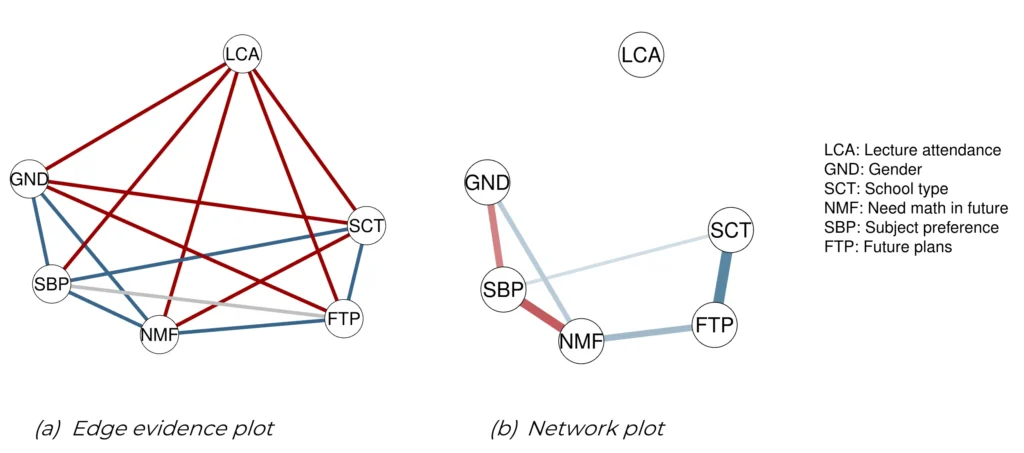
- This user-friendly package streamlines the entire workflow, from fitting models and extracting key results to creating publication-ready plots with just a few lines of code.
- To further lower the barrier to entry, easybgm includes educational vignettes that guide researchers through the process of Bayesian analysis, helping to bridge the gap between complex statistical methods and practical application.
Keywords: