Introduction
Network psychometrics is an increasingly popular approach to modeling the statistical relations between psychological constructs or behavioral measures (Epskamp, 2017). In this approach, the relations between measures are represented as a network, with each node of the network corresponding to a different construct (e.g, a symptom of a clinical disorder, or facet of a personality inventory), and directed/undirected edges corresponding to some kind of statistical relation (e.g., a partial correlation, directed temporal relation). Because of this network representation, researchers can apply statistical models and techniques from network science and graph theory to characterize the relative importance of individual variables. In the field of psychopathology, where the network psychometric approach is widely applied, nodes within a network typically correspond to individual observable symptoms. Assessing the importance and position of a symptom within a network of individual symptoms has immediate applications to psychological intervention design and evaluation. Another advantage to network psychometric models is that they are typically data driven, and therefore do not require a researcher to specify measurement and structural models before hand. These advantages have led to their proliferation in psychological and behavioral science in recent years (Costantini et al., 2019; Marsman, Borsboom, Kruis, Epskamp, van Bork, et al., 2018).
However, as an approach to studying psychopathology, network psychometrics has been criticized on a variety of theoretical and statistical grounds. The majority of these critiques pit the network psychometric approach against a more traditional latent variable modeling approach, and seek to inform the choice between the two different modeling frameworks. Significantly less work has been done in methodologically evaluating network psychometric methods as they are currently used and providing advice for future application. This kind of methodological evaluation is particularly important for the network psychometric approach, as it is a relatively new set of techniques to social science researchers, and does not have the same history of methodological evaluation the more traditional latent variable modeling framework has. A critical and as yet unanswered question regarding network psychometric models is: how robust are network psychometric approaches to common sources of measurement error and/or model misspecification, such as unreliable items or incomplete sets of variables? This question must be evaluated just as previously done with latent variable models. As network psychometric models will impacted by measurement error or model misspecification, applied researchers need to know if any estimation method is more or less robust to the effects of these issues. The present study aims to fill in such gap by examining the relative performance of two commonly used estimating methods for Gaussian Graphical Models, EBICglasso and LoGo-TMFG when applied to data afflicted by measurement error or omitted variables. Cross-sectional models are the focus of this study for two reasons: a) while temporal/longitudinal network models are becoming more widely used in psychological research, cross-sectional network models have been, and still are, frequently used to analyze pre-existing cross-sectional psychological data and b) measurement error and omitted variables are issues that can occur in both cross-sectional and longitudinal models, with cross-sectional models providing a simpler evaluation case than longitudinal models.
The remainder of this article is structured as follows: first, we briefly examine the contrast of latent variable modeling and network psychometric approaches in the current literature and discuss how this contrast, when used to provide methodological evaluation on network psychometric approaches, fails to reveal actionable insight into the use of network psychometric methods. Second, we discuss omitted variables and unreliable items in the context of Gaussian Graphical Models (Epskamp, Waldorp, et al., 2018; Lauritzen, 1996). Next, we describe our simulation approach, which allows us to compare the performances of two commonly used estimation methods for GGMs, EBICglasso (Epskamp, 2017) and LoGo-TMFG (Barfuss et al., 2016) under conditions of measurement error and omitted variables. Finally, we summarize our findings and contextualize our results for applied researchers in psychopathology.
Latent Variable vs. Network Psychometric Approaches
In Bringmann & Eronen (2018) the authors discuss how literature both for and against a network psychometric approach to psychopathology has been rooted in a false dichotomy between common cause and network psychometric models. Prima facie, these two conceptual frameworks are seemingly at odds with one another. A common cause framework, which is often operationalized with latent factor models, suggests that the observable symptoms of mental disorders are caused by an underlying common factor (i.e. depression as a latent entity that causes the symptoms of major depressive disorder). The network psychometric framework proposes that mental disorders are consistent sets of symptoms, problems and behaviors that causally interact over time (i.e. fatigue, a central symptom of depression, causes difficulty concentrating, which then causes anxiety and associated coping behaviors, which lead back to increased fatigue) (Borsboom & Cramer, 2013). However, when considering the statistical models used to represent these conceptual frameworks, as Bringmann and Eronen point out, the apparent dichotomy is misleading. The statistical models used to represent network or common cause conceptual models are in fact flexible enough to admit a spectrum of models that span from a purely network representation of psychological disorders to a purely common cause representation. For example, latent variables can be included in network models (Anandkumar et al., 2013; Van Der Maas et al., 2017) and latent variable models can have network components (Epskamp et al., 2017). To further show that the dichotomy is misleading, in several cases it has been shown that network models are statistically equivalent to common cause models, with Marsman, Borsboom, Kruis, Epskamp, Van Bork, et al. (2018) showing equivalences between the Ising model and multidimensional IRT models, and Waldorp & Marsman (2022) showing equivalences between unidimensional latent variable models and dense GGMs. This mixing of (fundamentally equivalent) statistical frameworks with the motivating (and highly contrasting) conceptual frameworks has led to several articles that compare and contrast inference under assumptions of incorrect conceptual models, e.g. fitting a network model when the assumed generating process is a common cause model (e.g., Hallquist et al., 2019) or provide conceptual contrasts between the two modeling frameworks (e.g., Fried & Cramer, 2017). While this work is useful in informing the debate between the network and common cause conceptual frameworks, this is less useful in evaluating how well different major network estimation methods perform under realistic data conditions. An evaluation of how different prominent network estimation methods perform under realistic data conditions would help guide researchers in choosing an estimation technique for their own analyses.
Gaussian Graphical Models
The current investigation adopts a commonly used framework to fit cross-sectional network psychometric models, Gaussian Graphical Models. Gaussian Graphical Models (Epskamp, Waldorp, et al., 2018; GGM Lauritzen, 1996), at their core, are network representations of the partial correlation matrix of a multivariate normal distribution. Let a \(p\) dimensional random variable \(\mathbf{X}\) be distributed as a 0-centered multivariate normal variate with covariance matrix \(\boldsymbol{\Sigma}\). Let \(G\) be an undirected network with \(p\) vertices, and an edge set denoted as \(E\). The random variable \(\mathbf{X}\) is said to follow a Gaussian Graphical Model with graph \(G\) if
\(\begin{equation*}\boldsymbol{\Sigma}^{-1}_{ij} = 0\text{ } \forall(i,j) \notin E.\end{equation*}\)
In other words, GGMs are, in most use cases, sparse representations of the conditional relations between pairs of variables. Note, this is where GGMs differ from simply computing the partial correlation matrix of \(\mathbf{X}\). The partial correlation matrix, as computed by the appropriately standardized inverse sample covariance matrix, will be dense, in that every estimated relation between pairs of variables will be non-zero. This corresponds to a GGM with a dense underlying graph, but a GGM need not be dense. The utility in using a GGM is the ability to estimate a sparse partial correlation matrix, in that some partial correlations will be shrunk to 0, and therefore not needed to be estimated. This sparsity allows for a more parsimonious representation of the conditional relations between the variables under study.
Furthermore, GGMs represent Pairwise Markov Random Fields (Epskamp, Waldorp, et al., 2018). This property says that non-adjacent variables (i.e., variables that do not share an edge) are conditionally independent of one another given all other variables in the network. The conditional independence of non-adjacent variables has important interpretational implications, in that if one’s set of psychological variables are normally distributed, and the GGM is correctly specified, the resulting sparse network of partial correlations fully represents the unique relations between the variables in the network.
Due to their ease of interpretability (being sparse partial correlation matrices) and estimation, GGMs are commonly used in psychological sciences to estimate cross-sectional networks (Epskamp, Waldorp, et al., 2018). The two methods for estimating GGMs that the current paper focuses on are a regularization based approach termed EBICglasso (Foygel & Drton, 2010) and an information filtering approach termed LoGo-TMFG (Local/Global – Triangulated Maximally Filtered Graph; Barfuss et al., 2016). Both approaches result in an estimate of a sparse inverse covariance matrix (i.e., when appropriately normalized a sparse partial correlation matrix).
EBICglasso uses regularization approaches (i.e., graphical LASSO, Friedman et al., 2008) to induce sparsity, and uses a search procedure that attempts to determine the optimal regularization parameter that minimizes the extended BIC or BIC (Foygel & Drton, 2010). This in turn allows analysts to estimate a sparse GGM that balances both parsimony and fit to the data. However, EBICglasso, using regularization is known to result in biased estimates of the inverse covariances. Given its ease of use and R implementation, EBICglasso has been the standard method for estimating cross-sectional network psychometric models since its introduction.
The LoGo-TMFG (Barfuss et al., 2016) does not use regularization to induce sparsity, rather it begins with an empty graphical representation of the sparse inverse covariance matrix, and progressively adds and removes edges such that the connected cliques (i.e., sets of three nodes/variables) maximize the log-likelihood of the resulting inverse covariance matrix. Like EBICglasso, LoGo-TMFG results in consistent estimation of the sparse inverse-covariance matrix, but due to the lack of regularization, does not have the same a priori bias in coefficient estimation.
In the original paper introducing LoGo-TMFG (Barfuss et al., 2016), the authors demonstrated that their approach had equivalent or better performance than graphical lasso, with LoGo-TMFG resulting in higher log-likelihoods than cross-validated Glasso. However, the estimation of inverse covariance matrices, by either EBICglasso or LoGo-TMFG, is likely to be biased by common features of psychological data (i.e., measurement error). This bias will have unpredictable effects on any outcomes of interest based on the GGM, such as measures of centrality or topological network statistics, and as such is vitally important to assess the relative performances of these two approaches under measurement error and omitted variable bias.
Sources of Bias in GGMs
While there are many possible sources of bias in network psychometric models, in this article we focus on two sources that have been previously examined in the context of latent variable models, measurement error and omitted variables.
Measurement Error
Measurement error occurs when the “true” value of a variable cannot be directly observed. The observed value, \(X^*\), of a variable \(X\) is then of the following form:
\(\begin{equation} X^* = X + \epsilon\end{equation}\quad(1)\)
where \(\epsilon\) is random variable with \(\text{E}[\epsilon] = 0\) that is independent of \(X\) itself. The impact of unmodeled measurement error on a variety of statistical models has been a key topic of study in psychometrics since the very beginnings of the field. Early work by Lord et al. (1968) showed that unreliable test scores (i.e., test scores that are impacted by measurement error) lead to attenuated estimates of test-retest reliability. Attenuated estimates, or estimates that are biased towards 0, commonly occur when the estimate is of a relation between two measurement error impacted variables, but when using more complex statistical models the effect of measurement error quickly becomes unpredictable. For models like structural equation models with latent variables (Bollen, 1989; Gillespie & Fox, 1980; Rigdon, 1994; Rubio & Gillespie, 1995) and manifest variable path models (Cole & Preacher, 2014) measurement error might cause attenuation of effect estimates (bias towards 0) or inflation of effect estimates (bias away from 0), depending on which variables are impacted by measurement error.
This long history of methodological work also highlights three problematic aspects of unmodeled measurement error: 1) the magnitude of the bias induced by unmodeled measurement error is often large, leading to false positive and/or false negative hypothesis tests, 2) the severity of the impact of measurement error increases with model complexity (Cole & Preacher, 2014), and 3) increases in sample size does not reduce the effect of unmodeled measurement error and in many cases will lead to more spurious findings overall. It is difficult to overstate the potential negative impacts of unmodeled measurement error, and the only choices for how to handle it are either by using perfectly reliable measures (a virtual impossibility in psychopathology and in psychology at large) or by explicitly modeling it. However, this second option requires additional sources of information. For example, it is possible to correct for unreliable test scores if one knows from previous research how unreliable a given test is. The use of latent variable models for accounting for measurement error requires the observation of several indicators of the unobserved variable. This is to say, if the study design itself did not collect the information needed to correct for measurement error, then no amount of model fitting or different estimation techniques will fully remove the bias induced by measurement error.
Gaussian graphical models, as previously described, are estimates of the partial correlations between the observed measurements, which implies that if the items modeled by a given GGM are impacted by measurement error, then the resulting GGM will be biased. Liu (1988) showed analytically how measurement error can impact partial correlation estimates. Given a partial correlation \(\rho(X, Y | Z )\), if only \(X\) and \(Y\) are unreliable, then the partial correlation will be attenuated. If the measurement error occurs only in \(Z\), then the partial correlation will be inflated. Finally, if the measurement error occurs in all the variables, then the resulting bias will be unpredictable, depending on the relative amounts of error in each variable. More recent work by Neal & Neal (2023) shows that, for psychometric networks with only single item indicators, the impact of measurement error can be quite severe, lessening only with an increased sample size. Additionally, they demonstrated that using multiple indicators in a latent variable network psychometric model (Epskamp et al., 2017) can drastically reduce the impact of measurement error on the estimation of the underlying network.
The properties of partial correlations have major implications for the performance of GGMs under conditions of measurement error, and this is particularly concerning given that network methods are meant to be used to assess large, highly complex systems of variables. Finally, the potential impact of measurement error on the bias of individual partial correlation estimates is particularly concerning from a network statistic standpoint. Many outcomes of network psychometric models involve statistics calculated from the estimated network itself (i.e., centrality metrics that describe the importance of a given symptom). These network statistics are complex functions of the underlying network, which implies that bias in the estimates of the partial correlation will lead to unpredictable bias in the estimates of the network statistics. Additionally, while the impact of measurement error is known analytically for estimation of dense partial correlation matrices, it is less apparent how measurement error will impact algorithms that estimate sparse partial correlation matrices (such as EBICglasso and LoGo-TMFG). However, regardless of the impacts of measurement error, the solution is the same for network models as it is for any other class of models: increase sample size, use better measures, or explicitly account for measurement error. For network psychometric models, explicitly accounting for measurement error can be accomplished using a latent variable network approach (Epskamp et al., 2017), which can be used with a mix of single item indicators and multiple indicators as needed.
Omitted Variable Bias
Omitted variable bias occurs when an important predictor to explain the variability of the outcome is left out of the model, leading to a correlated outcome and model residual, as well as biased parameter estimation of the other predictors in the model. This is best illustrated with a simple linear model:
\(\begin{equation}Y = \beta_1 X_1 + \beta_2 X_2 +\epsilon_1\end{equation}\quad(2)\)
where the relation between \(X_1\) and \(X_2\) can be described by \(X_2 = \gamma X_1 + \epsilon_2\), with both \(\epsilon_1\) and \(\epsilon_2\) being normally distributed with an expected value of 0. If \(X_2\) is omitted from the first equation, then the estimated model becomes:
\(\begin{equation}Y = (\beta_1 + \gamma \beta_2)X_1 +(\epsilon_1 + \beta_2\epsilon_2)\end{equation}\quad(3)\)
which implies that the estimated \(\beta_1\) when \(X_2\) is omitted is biased by a factor of \(\gamma \beta_2\). This can be extended to the case of the GGM, as GGMs can be reparameterized as a set of linear regression equations. More broadly, the omission of variables from Pairwise Markov Fields leads to the resulting sub-graph no longer being pairwise Markov (Eq.5, Epskamp, Maris, et al., 2018). In terms of substantive inference, this implies that if a relevant variable, be it a symptom or a behavioral measure, is excluded from the estimation of the GGM, then pairwise relations between variables are no longer able to be interpreted as wholly specific to the pair in question. Rather, the relations become contaminated by the shared variance of the omitted variable.
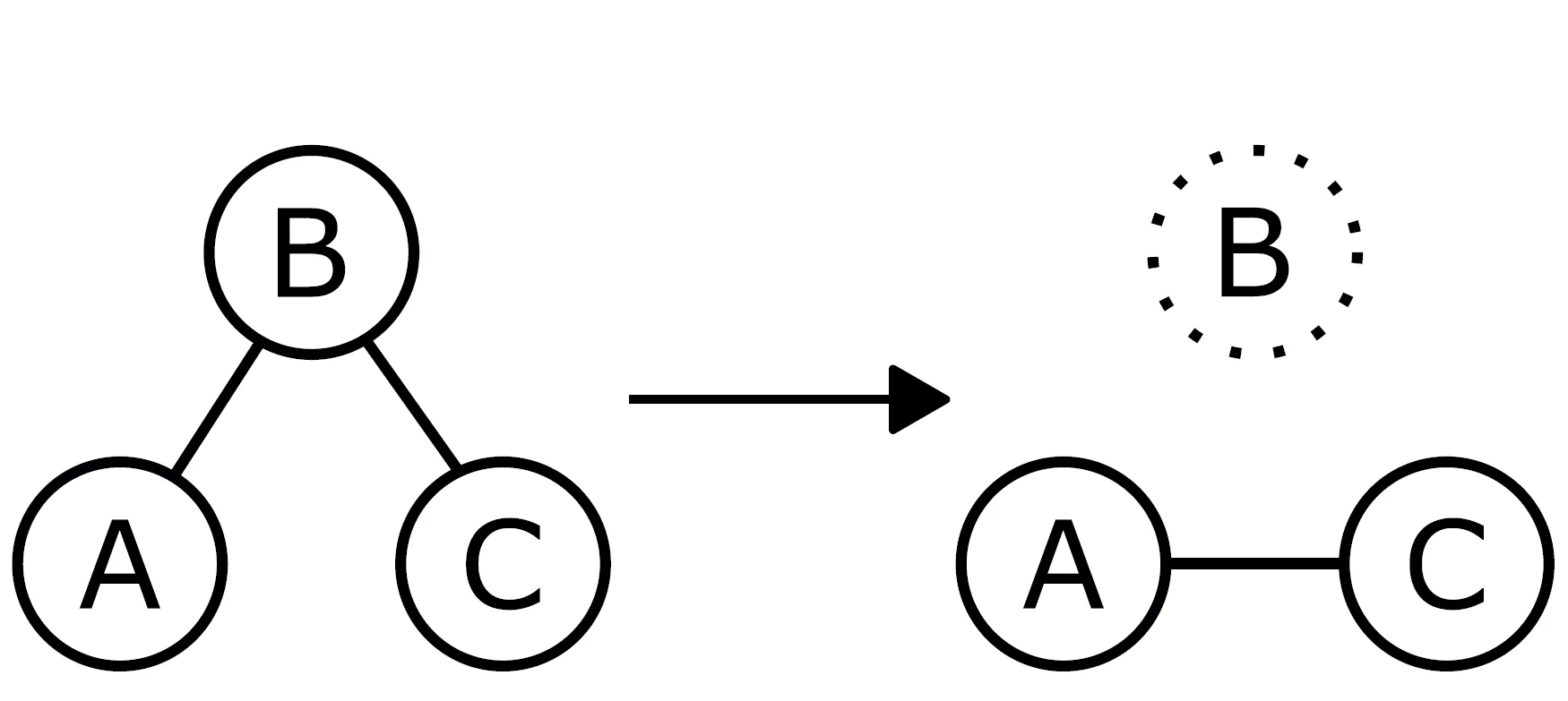
There is a related and applicable issue that is often raised in social network research: the boundary problem (Laumann et al., 1989). In social networks, the boundary problem refers to the issues arising when one fails to collect the relation data from individuals that are relevant to the individuals already present in the network. For example, if one is studying the relation between an individual’s social network centrality (as a measure of social engagement) and psychological wellbeing, and only collect the social relations from a specific social setting (e.g., the workplace), then your measures of centrality will be inaccurate if a given individual has social relations not in that social setting (i.e., they have no friends in the workplace, but many friends outside of the workplace). Neal & Neal (2023) recently extended this issue to psychometric networks, noting that if you are calculating the centrality of a psychological construct, and fail to measure other psychological constructs that are related to the original construct, then necessarily the estimates of centrality will be in some sense inaccurate. However, unlike in social networks where failure to measure relevant social ties from some setting will not impact the measurement of social ties in the collected setting, the omission of relevant variables in psychometric networks will change the estimates of edges between measured variables as well, at least when the psychometric network is estimated using a conditional association metric such as partial correlations. For example, consider the example shown in Figure 1. There, the original network shows estimated conditional relations (i.e., partial correlations) between variable A and B, and between B to C. If variable B is omitted, and the network is re-estimated, then a spurious association between A and C is found. This in turn will lead to biased estimates of node centrality measures (in addition to the bias caused by not having any association information on the variable B).
Figure 1
The Impact of Omitted Variables on Network Estimation. The omission of variable B leads to the estimation of the spurious relation between A and C.
We must emphasize the pernicious nature of the omitted variable problem, and note that, as with measurement error, omitted variables will impact the estimation of other model types, such as more traditional latent variable models. However, as network models tend to be more flexible and less constrained than other approaches, the effects of omitted variables are less predictable and potentially worse than the effects would be for a different modeling approach. There is no one solution to this problem other than the one described by Neal and Neal (2023): collect all the relevant variables within a reasonable theoretical boundary.
An Empirical Example
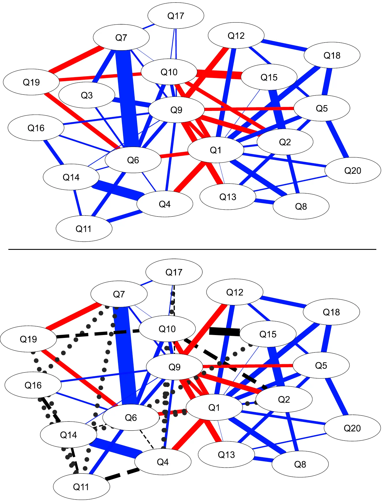
To demonstrate these issues in the estimation of cross-sectional networks, here we present a brief empirical example using Open Psychometrics Project’s Machiavellianism dataset (Open Psychometrics Project, 2024). The MACH-IV scale (Christie & Geis, 1970) consists of 20 items that measure the personality trait of Machiavellianism, the tendency to use others for your own ends. This scale uses 5 point Likert responses. For this example, we randomly sampled 1000 observations from the 73,489 available responses, and estimated the psychometric network of the items using the LoGo-TMFG method, as this method accounts for the ordinal response scale. We then removed each item from the dataset in turn, re-estimating the network and calculating the missing edges, false positive edges and the relative bias of edge weight estimates. Removal of variables led to a range of impacts. Several items’ removal had no impact on the presence or absence of edges and led to minimal bias (relative bias of ∼ .02 − .03). On the most extreme side of impact, the removal of Q3 “One should take action only when sure it is morally right.” led to a sensitivity rate of .82 (9 edges were missing), a specificity rate of .93 (9 edges were erroneously estimated) and a relative bias in edge weight of .126. A visualization of the network before and after the removal of Q3 is presented in Figure 2.
This empirical example demonstrates the wide ranging impacts of variable omission, and we expect that the effects of measurement error would be similar, differing only in how extreme the impact would be. However, it is unclear how the different topological features of the omitted variables (i.e., how central a variable is) relate to the induced bias. The following simulation study evaluates both the performance of the two estimating methods, as well as how node centrality relates to the impact of omission/mismeasurement.
Figure 2
Psychometric Network of MACH-IV Scale. Top Panel: Full Scale. Bottom Panel: Scale with Q3 removed. Edge thickness represents partial correlation magnitude. Red edges are negative associations, blue edges are positive associations. Dashed black lines are edges that are not detected once Q3 was removed. Dotted black lines represent false positive edges that are estimated only when Q3 was removed.
The Current Study
Motivated by the previous concerns, our study sought to understand which approach, EBICglasso or LoGo-TMFG, is more robust to the effects of measurement error and omitted variables. As it is the case that measurement error and omitted variables will result in the estimation of a biased network (this is evident from how measurement error and omitted variables effect linear models more generally), it is important to determine under what conditions and for what outcomes each of the estimation approaches is superior. Specifically, we were interested in the impact of measurement error and omitted variables on direct measures of model recovery such as sensitivity and specificity of edge recovery, and the relative bias of edge weights. In addition, our study also aimed to understand the extent to which the properties of specific nodes (i.e., the true centrality of a node) relate to the impact of its removal or imprecise measurement.
Towards this end, we designed a simulation study whose generating processes are wholly within the conceptual framework of network psychometrics. Specifically, we generated a series of directed networks representing a variety of causal structures, and used those causal generating networks to simulate our cross-sectional data. This matches the conceptual data generating process proposed by the network psychometric framework, in that observations are generated by a dynamic system of interacting variables, rather than common causes generating the indicators (Borsboom & Cramer, 2013). Another advantage of this simulation design is that we could obtain ground truth values of both the network structures and of subsequently derived network statistics, allowing us to assess the objective performance of the GGM framework in recovering the true network model. Finally, using ground truth network models allowed us to compute ground truth nodal centrality measures, which were then used to quantify the effect of node removal/mis-measuring. This allowed us to better map onto the conceptual framework of the network psychometric approach, in that the complexity of the relations between variables in the network is precisely what the network psychometric approach seeks to evaluate.
We hypothesized that the removal or mis-measuring of highly central nodes would lead to the largest increase in bias when examining edge recovery (sensitivity/specificity) and edge strength. Our hypothesis is based on the fact that highly central nodes are, by definition, strongly related to many other nodes in the network, and therefore their omission or mis-measuring would likely have a more severe impact on the overall network structure than the removal of a node that was less central. Second, network statistics based on geodesics are highly dependent on the overall topology of the network, and the removal or mis-measuring of a highly central node would likely have a strong impact on the overall topology/structure of the network.
Given LoGo-TMFG’s performance relative to Glasso in Barfuss et al. (2016), we hypothesize that it will be overall less impacted by measurement error and omitted variables. However, we have no specific hypothesis as to how node centrality will moderate the performance. There are two reasonable scenarios to consider. First, LoGo-TMFG could be uniformly better than EBICGlasso across the range of nodal centrality values. Second, nodal centrality could moderate performance such that injecting measurement error/omitting a highly central variable results in a larger discrepancy in performance than doing the same to a non-central variable.
Simulation Study
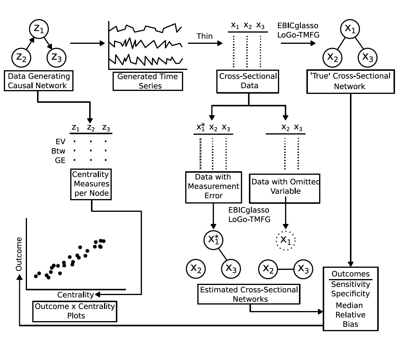
We conducted all aspects of the simulation study in R (R Core Team, 2020). A flowchart describing the entire simulation design can be found in Figure 3 below.
Figure 3
Simulation Flowchart. Note that the outcomes are calculated by comparing the estimated cross-sectional networks with the ‘true’ cross-sectional networks. Additionally, the comparison between EBICglasso and LoGo-TMFG with respect to the outcomes is not depicted in the flowchart.
Data Generating Models
To better map onto real world data generating processes, we first simulated a series of sparse directed network models which were then used to simulate cross-sectional data.
These sparse directed models correspond to VAR(1) models of the following form
\(\begin{equation}z_{t+1} = \mathbf{A}z_t + \epsilon \text{ with } \epsilon \sim MVN(0, \mathbf{I}_p)\label{eq:var1}\end{equation}\quad(4)\)
where \(z_{t}\) is a \(p\) length vector of real numbers, \(\mathbf{A}\) is a \(p \times p\) matrix of lag-1 coefficients and \(\epsilon\) is multivariate normal white noise with a identity covariance matrix.
The above model corresponds to the situation where all causal relations operate at lag-1 (i.e., from time t to t+1), and there is no measurement error present (i.e., z is observed time series). The identity covariance matrix of \(\epsilon\) represents the case where there are unmeasured causes for each variable (variances of 1), but these causes are unique to each variable (off diagonal entries of 0). This represents the ideal case when it comes to a causal model, but specifying an ideal generative model allows us to best evaluate the impact of measurement error and omitted variables on resulting inference. Use of a directed causal model as our data generating process also allows us to evaluate the impact of measurement error/omitted variables with respect to nodal network statistics calculated on the generative directed network.
\(A\) matrices of a given dimension \(p\) and density \(d\) were generated with the following steps.Algorithm 1: Generating Random Stationary Directed Networks
- For each \(i \in 1 \text{ to } p\), sample \(\mathbf{A}_{ii}\) from Uniform(0,.8). This corresponds to autoregressive effects.
- Randomly chose an \(ij\) pair such that \(\mathbf{A}_{ij} = 0\) and \(\mathbf{A}_{ji} = 0\). Sample \(\mathbf{A}_{ij}\) from Uniform(-.8,.8). Repeat until \(\mathbf{A}\) reaches the target density \(d\).
- Check the eigenvalues of \(\mathbf{A}, \lambda(\mathbf{A})\). If all \(\lambda(\mathbf{A}) < 1\) continue to next step, else reject \(\mathbf{A}\) and return to Step 1.
- Check if \(\mathbf{A}\) is fully weakly connected (i.e., when directionality of paths is ignored, \(\mathbf{A}\) has 1 connected component.) If \(\mathbf{A}\) is not fully weakly connected, reject \(\mathbf{A}\) and return to Step 1.
This generative process ensures that \(\mathbf{A}\) has several desirable properties. Step 2 together with the identity covariance matrix ensures that the resulting generative model has no bidirectional effects, which allows us to avoid considering bias due to simultaneity. Step 3 ensures that the VAR(1) model specified in Eq. 4 is weakly stationary. Step 4 ensures that the model implied asymptotic covariance matrix is not block diagonal (which leads to the resulting network being completely connected).
Our interest in this manuscript is to evaluate the impact of measurement error and omitted variable bias on network psychometric models applied to cross-sectional data. However, the generative model above is for temporally dependent data. To use this model to generate cross-sectional data, we thinned the generated temporal data to remove the temporal dependency. To sample \(n\) observations from a model described in Eq. 4, we generated \(n\times 20\) timepoints and retained every 20th timepoint. This results in a collection of independent observations (in that the auto-correlation at lag 20 is approximately 0) that were all generated by the same directed model. To delineate this subset of observations that serve as our cross-sectional data from the full generated timeseries \(\mathbf{z}\), we use \(\mathbf{x}\) and index using \(i\).
A reasonable question that a reader might pose here is: If your interest in is cross-sectional data, why generate temporally dependent data and thin, when one can generate cross-sectional data directly from a model implied covariance matrix constructed by, for example, the corresponding confirmatory factor model? The answer to this question is twofold: First, generating data from a model implied covariance matrix requires one to specify the model that results in the implied covariance matrix. If we were to specify a confirmatory factor model and generate data from that model, we only have one example of a covariance structure. Our approach allows us to simulated across the population of cross-sectional covariance matrices, as we are sampling from the population of admissible temporal network models using Algorithm 1. This approach in turn results in a wide range of nodal statistics, drawn from networks with differing structures. This allows our results to be generalizable across a family of data generating models, rather than being restricted to one or a handful of data generating structural models. Second, while directly sampling from the population of correlation matrices is possible using an algorithm like that of Joe (2006), this approach results in randomly sampled correlation matrices that are less structured than what would be found in psychological data. Whereas sampling from the space of admissible VAR(1) models and using those models to generate our cross-sectional data results in cross-sectional network structures that are more generalizable to what might be found in psychological studies.
Omitted Variable Bias and Measurement Error
\(\mathbf{X}\) represents an ideal cross-sectional sample where no measurement error is present, and no variable is omitted. To simulate the impact of an omitted variable, we simply omit each variable in turn. This creates a series of datasets denoted \(\mathbf{X}_{-i}\) where \(i\) ranges from 1 to \(p\).To simulate the impact of random measurement error, we add differing amounts of independent normal noise to each variable in turn. We define the amount of measurement error as the proportion of variance in the final transformed (i.e., measured with error) variable \(x^*\). First, let \(m\) be the target proportion of measurement error. We calculate the standard deviation of the generated error as \(\sigma = \sqrt{\frac{m\text{Var(x)}}{1-mError}}\). \(x^*\) is then defined as
\(\begin{equation}x^* = (x + \gamma)\sqrt{\frac{\text{Var}(x)}{\text{Var}(x)+\sigma^2}}\end{equation}\)
where \(\gamma \sim N(0, \sigma^2)\).
This results in the variable \(x^*\) having the same variance as the original \(x\) while \(m\) proportion of that variance is now independent measurement error.
Comparing Estimated Sparse Partial Correlation Matrices Against a Sparse “Ground Truth” Partial Correlation Matrix
The outcomes of this study (described in detail below), are the sensitivity and specificity of edge detection, as well as the bias in coefficient estimation. However, our data generating process does not produce sparse ground truth partial correlation matrices. Rather, the generating model implied partial correlation matrix is dense, which makes the calculation of sensitivity and specificity impossible. To provide a comparable “ground truth” network to calculate sensitivity and specificity against, we apply EBICglasso and LoGo-TMFG to the complete cross-sectional dataset, before adding measurement error or omitted variable bias.
Simulation Conditions
Data was generated with the following full cross of design factors:
- Number of Variables/Density: 20 nodes at .2 edge density (i.e., the proportion of non-0 edges) and 10 nodes at .2 edge density.
- Number of Observations: 200 and 1000 observations.
This cross of design factors resulted in 4 cells: 20 variables and 200 observations, 20 variables and 1000 observations, 10 variables and 200 observations, and 10 variables and 1000 observations. For each of these 4 cells, 50 networks were generated, and for each of those 50 networks, 100 cross-sectional datasets were generated. This resulted in 4 x 50 x 100 = 20000 raw datasets generated.
Omitted variable bias was evaluated by removing each variable in turn, resulting in 20 omitted variable datasets for the 20 variable networks, and 10 omitted variable datasets for the 10 variable networks.
Measurement error was assessed at three levels, .25 (light), .5 and .75 (heavy) proportion of a variable’s variance. Measurement error was only applied to a single variable at a time, resulting in 20 x 3 measurement error datasets for the 20 node networks, and 10 x 3 measurement error datasets for the 10 node networks.
Finally, the network edge density was set at .2 to strike a balance between generating weakly connected networks with reasonable numbers of edges, and generating networks that result in inadmissable (i.e., non-stationary explosive) data generation.
Estimation Approaches
For EBICglasso, we used the implementation contained in the R package qgraph (Epskamp et al., 2012). For tuning parameters, we set \(\gamma = .5\) (the default value for the function), and set thresholding to true. Here, thresholding is a step that sets small estimated correlations to 0, which increases specificity, and provides an additional means of sparsification. For LoGo-TMFG, we used the implementation in NetworkToolbox (Christensen, 2019). This method has no tuning parameters.
Evaluating Outcomes
Centrality of Nodes as Predictors of Network Outcomes
To better interpret the impact of an omitted variable or measurement error in the context of network models, we calculate the centrality of the manipulated variable based on the directed model network \(\mathbf{A}\), because these metrics directly correspond to how important a given variable is with respect to the overall network. Specifically, we calculate the following for each node
- Eigenvector Centrality – A measure of how strongly connected a node is to the rest of the network. This metric is related to strength and degree, but upweights centrality when nodes are connected to other highly central nodes (Bonacich, 1987).
- Betweenness Centrality – Calculated as the number of shortest paths that pass through a given node, this measure reflects how well a node connects unconnected regions of a network (Freeman, 1977).
- Nodal Efficiency – Calculated as the average inverse shortest path from a given node to all other nodes. Related to closeness centrality, but is calculated on the inverse edge strength (to reflect that high values of edge strength represent greater connections as opposed to greater distance or cost) (Latora & Marchiori, 2001).
This allows us to evaluate the impact of omitting or mis-measuring a highly central variable on the resulting estimates of the cross-sectional network. Note that these centrality measures are not used as outcomes in this simulation study, rather our interest is in how the original centrality of a given node relates to the impact of omitting or miss-measuring that node.
As these network statistics are continuous in nature, in order to report outcomes we applied a Gaussian kernel smoother at the mean network statistic, and at +1SD above and below the mean network statistic. The SD of the Gaussian kernel was calculated to be .25SD of the given network statistic.
Simulation Outcome Measures
Sensitivity and Specificity
Sensitivity is the proportion of non-zero edges correctly recovered, while specificity is 1 minus the percentage of zero-edges (i.e., non-present edges) incorrectly estimated as non-zero. Perfect recovery of the structure corresponds to a sensitivity and specificity of 1. These are commonly used measures when evaluating the performance of network estimation procedures in both psychology and neuroimaging.
Median Relative Bias
Median relative bias is the median relative difference between weight estimates in the original unmanipulated network and the weight estimates in the manipulated network. This value was calculated using those edges that were a) could occur in the manipulated network and b) were non-zero in the original network.
As relative bias is examined across the entire network, we use the median relative bias to avoid being impacted by large outliers.
To compare EBICglasso and LoGo-TMFG, we computed the difference in outcomes between the two methods for each simulated dataset. This ensures an “apples-to-apples” comparison of performance, as each algorithm is applied to the same dataset (with the same measurement error/omitted variable). As we calculated this difference as Outcome𝐸𝐵𝐼𝐶𝑔𝑙𝑎𝑠𝑠𝑜 − Outcome𝐿𝑜𝐺𝑜, positive values of this difference indicate better performance for EBICglasso in the case of sensitivity and specificity, while negative values of this difference indicate better performance of EBICGlasso for relative bias
Results
Due to space considerations, we report only the findings for n = 200, and limit our figures to show only the outcome comparisons (i.e., the difference between EBICglasso and LoGo-TMFG) conditional on the eigenvector centrality of the targeted node. All other results (n = 1000 and marginal outcome values) are tabled in the Supplementary Information. Broadly speaking, the pattern of results is similar across different network statistics (i.e., omitting or miss-measuring a highly central variable tends to have greater impact on the performance).
Overall Performance
Overall performance is tabled in Tables S1-3, and the findings are summarized here. Across all node manipulations (omitting/mismeasuring), the negative impact of the manipulation (defined here as lower sensitivity/specificity and/or higher bias) was less for variables with lower than average centrality, and this effect was consistent for both EBICglasso and LoGo-TMFG. For both methods, omitting a variable resulted in a smaller negative impact on sensitivity than any of the measurement error conditions. This finding has a couple of minor exceptions, but is consistent across all network statistics. For specificity and bias, the omitted variable conditions tended to result in negative impacts similar to that of low amounts of measurement error. For the measurement error conditions, more measurement error resulted in greater negative impacts on outcomes. For overall specificity, EBICglasso showed greater than %95 specificity in all conditions, which is likely due to the use of thresholding. LoGo-TMFG does not maintain specificity across conditions, and shows the same pattern (more negative impacts the greater the centrality, more negative impacts the more measurement error is present.) Finally, comparing the 10 node results to the 20 node results, we see that using the 20 node networks resulted in better overall performance across all conditions, for both EBICglasso and LoGo-TMFG (with a few small exceptions).
Relative Performance
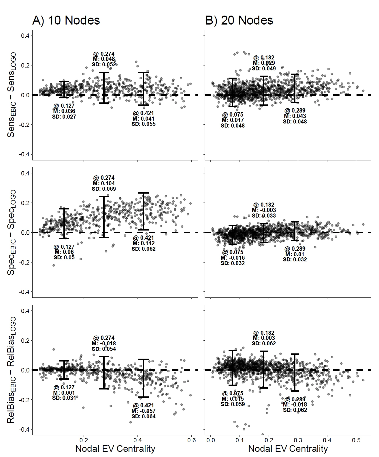
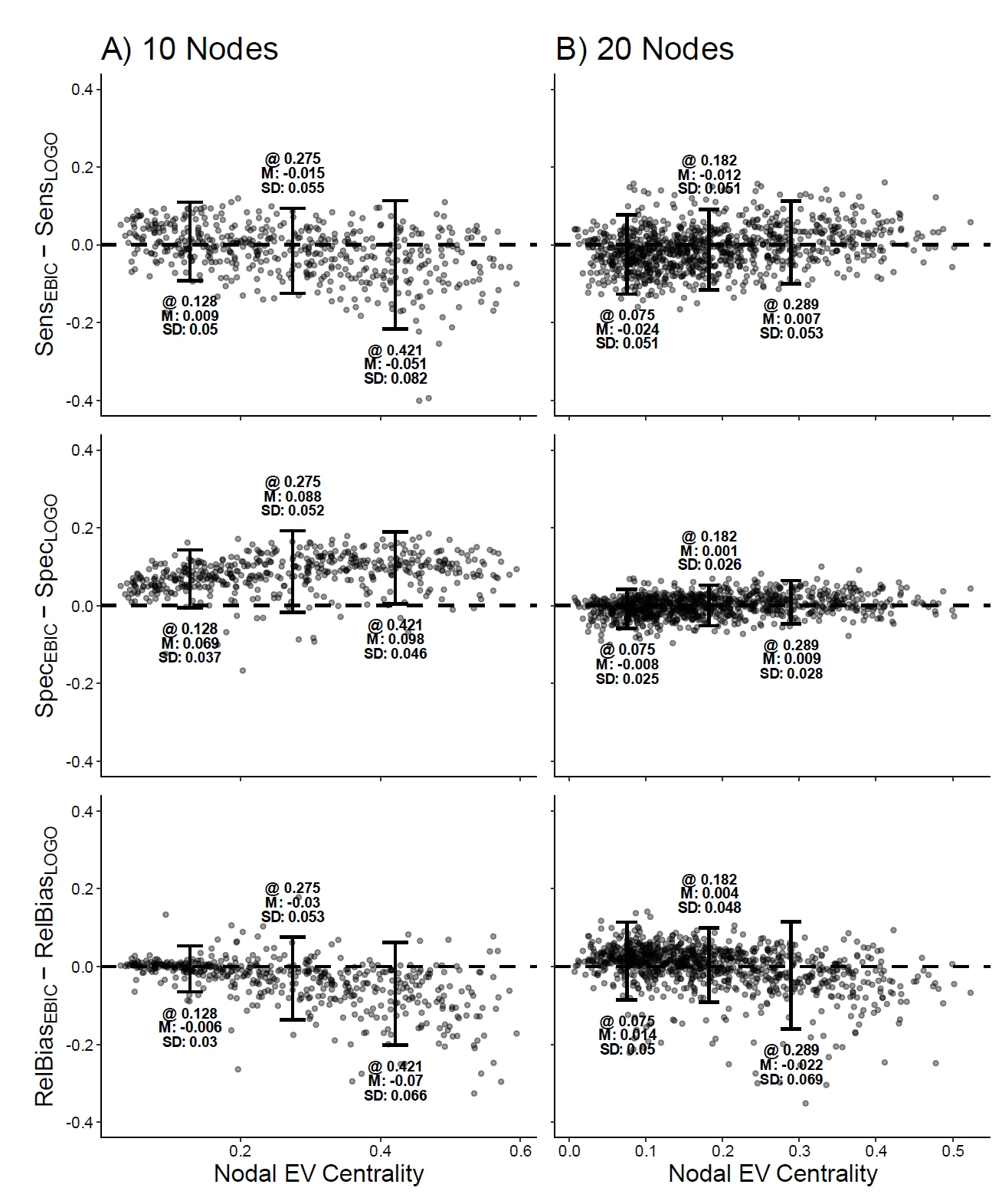
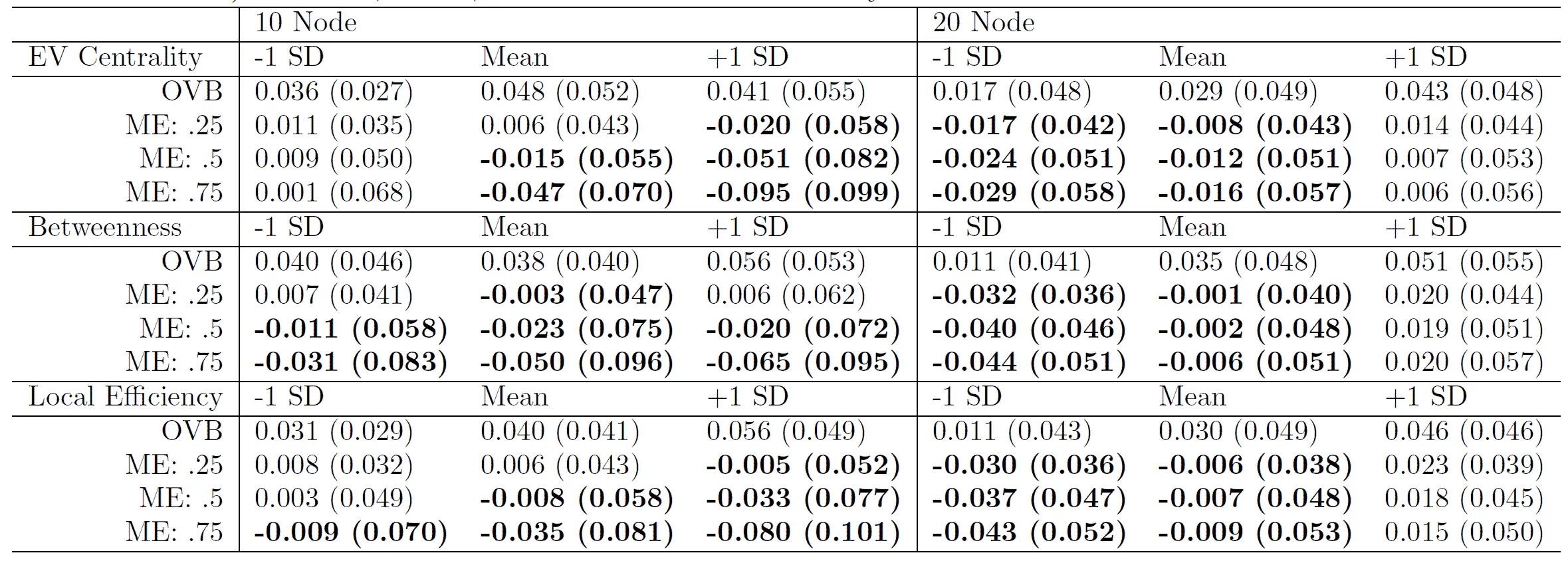
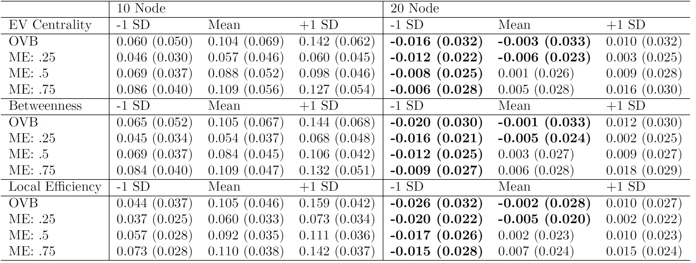
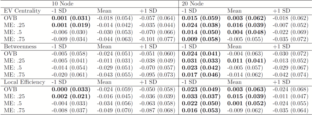
Tables 1, 2 and 3 show means and standard deviations for the comparisons between EBICglasso and LoGo-TMFG for sensitivity, specificity and bias respectively. Figures 4 and 5 plot the comparisons for sensitivity, specificity and bias in the omitted variable condition and measurement error of .5 condition respectively.
For sensitivity (Table 1), several patterns of findings emerge: First, in both the 10 and 20 node networks, LoGo-TMFG never outperforms EBICglasso when the variable is omitted, and, on average, EBICglasso performs better the more central the node is. These gains are fairly small, and accompanied by standard deviations that are of similar values to the expected value, suggesting that while the general tendency is that EBICglasso outperforms LoGo-TMFG, there is substantial variability in that performance and that there are datasets where LoGo-TMFG will outperform EBICglasso.
Figure 4
Comparison between EBICglasso and LoGo-TMFG for Sensitivity, Specificity and Bias by Eigenvector Centrality of the Omitted Variable (n = 200) Interval bars are shown at the mean value of nodal EV centrality, as well as +1SD from the mean. Graph annotations denote @ value of nodal EV centrality, M: kernel smoothed mean of comparison at that value of nodal EV centrality, and SD: kernel smoothed standard deviation of comparison at that value of nodal EV centrality. Interval bars span 2 x kernel smoothed SD.
Figure 5
Comparison between EBICglasso and LoGo-TMFG for Sensitivity, Specificity and Bias by Eigenvector Centrality of the Omitted Variable (n = 200) Interval bars are shown at the mean value of nodal EV centrality, as well as +1SD from the mean. Graph annotations denote @ value of nodal EV centrality, M: kernel smoothed mean of comparison at that value of nodal EV centrality, and SD: kernel smoothed standard deviation of comparison at that value of nodal EV centrality. Interval bars span 2 x kernel smoothed SD.
However, when the variable is contaminated with measurement error rather than being omitted all together, a different pattern for sensitivity is seen: For the 10 node networks, LoGo-TMFG has a small tendency to outperform EBICglasso when the centrality of the mis-measured variable is high, and that this out-performance increases with increasing amounts of measurement error. Here, the mean values of the performance can be fairly substantial (e.g., at +1 SD eigenvector centrality, LoGo-TMFG outperforms EBICglasso in sensitivity by .051 and .095 on average in the ME: .5 and ME: .75 conditions respectively). That being said, these mean values are always accompanied by large standard deviations, again suggesting that while on average, LoGo-TMFG will outperform EBICglasso, there are datasets where EBICglasso will perform better with respect to sensitivity.
Importantly, the findings with respect to the measurement error conditions are reversed in the 20 node condition: As nodal centrality becomes higher, EBICglasso tends to outperform LoGo-TMFG. Again, the mean values of the relative performance are small with large standard deviations, but this suggests that more variables in the psychometric network might improve EBICglasso’s performance relative to LoGo-TMFG’s performance with respect to sensitivity.
Specificity (Table 2) shows a distinct pattern of findings that are markedly different from that of sensitivity. In the 10 node condition, EBICglasso uniformly outperforms LoGo-TMFG, with the relative performance increasing with nodal centrality. Here, the standard deviation is small relative to the mean value, suggesting that EBICglasso consistently outperforms (with respect to specificity) LoGo-TMFG in all 10 node networks. This pattern of findings is likely due to the use of the thresholding functionality in EBICglasso, which scales with the number of predictor variables. However, the uniform better performance of EBICglasso disappears when moving to the 20 node networks. There, LoGo-TMFG tends to have slightly better performance when nodes have lower than average centrality, while EBICglasso tends to perform slightly better when nodes have higher than average centrality. These mean comparisons have relatively large standard deviations, which suggests that for specificity in the 20 node networks, EBICglasso and LoGo-TMFG have comparable performances.
Finally, for median relative bias (Table 3), EBICglasso tends to have equivalent performance or outperforms LoGo-TMFG across all 10 node conditions. While the mean relative performances do tend to have larger standard deviations, when nodal centrality is large, EBICglasso shows a clear advantage. However, this advantage disappears when considering the 20 node networks. There, like with specificity, LoGo-TMFG had slightly better on average performance when the nodal centrality was below average, while EBICglasso tended to have slightly better performance on average when nodal centrality was higher than average. Like with specificity, the standard deviations were high relative to the differences in performance, which suggests that EBICglasso and LoGo-TMFG tended to perform similarly in the 20 node conditions.
Table 1
Sensitivity Comparison at n = 200. Cell values are means (SD). Bolded entries show where LoGo outperformed EBICGlasso. Outcome values are calculated as Gaussian Kernel smoothed averages (see Section 2.6.1 for details) at -1SD, Mean, and +1SD of the centrality values
Table 2
Specificity Comparison at n = 200. Cell values are means (SD). Bolded entries show where LoGo outperformed EBICGlasso. Outcome values are calculated as Gaussian Kernel smoothed averages (see Section 2.6.1 for details) at -1SD, Mean, and +1SD of the centrality values.
Table 3
Median Relative Bias Comparison at n = 200. Cell values are means (SD). Bolded entries show where LoGo outperformed EBICGlasso. Outcome values are calculated as Gaussian Kernel smoothed averages (see Section 2.6.1 for details) at -1SD, Mean, and +1SD of the centrality values.
N = 1000 Findings
All results for our n = 1000 conditions are tabled in Tables S4-S6 for the comparisons between EBICglasso and LoGo-TMFG. Tables S7-S9 contain marginal results. The overall pattern of findings is very similar to what was seen in the n = 200 conditions: Both omitted variables and measurement error lead to reduced sensitivity/specificity and increased bias, these impacts increase with the amount of measurement error, and removal/mis-measuring of highly central variables leads to greater negative impacts on the outcomes. Notably, the magnitude of the marginal sensitivity, specificity and relative bias in the n = 1000 condition is close to the magnitude of the outcomes found in the n = 200 condition. For example, for median relative bias in the n = 200, the values range from ∼ .02 (in the case of omitted variables at low centrality) to ∼ .17 (in the case of heavily mismeasured variables with high centrality). The values in the n = 1000 conditions are nearly the same, which suggests that a larger sample does not mitigate the impact of omitted variables or measurement error.
As with the marginal results, the comparisons between EBICglasso and LoGo-TMFG are nearly identical to the n = 200 conditions. EBICglasso tends to have equivalent performance or outperform LoGo-TMFG for networks with 10 nodes, with EBICglasso’s advantages being particularly strong for highly central nodes. For the 20 node networks, EBICglasso and LoGo-TMFG show virtually equivalent performance, in that for any difference the standard deviation is of a similar magnitude. With respect to bias, LoGo-TMFG seems to perform better than EBICglasso in 20 node networks for low centrality nodes, but again, this effect is slight.
Discussion
The current study presents a detailed assessment on the robustness of two estimation methods for Gaussian Graphical Models, EBICglasso and LoGo-TMFG, to omitted variable bias and measurement error. The results of the simulation study suggested that, as expected, outcomes of the network psychometric models are sensitive to omitted variables or unreliable measurement. Specifically, the recovery rate of the correct edge presence (sensitivity), the rate of true negative detection (specificity), and the recovery of the correct edge value (median relative bias) were all negatively impacted by both omitted variables and unreliable measurement. This negative impact was consistent for both estimation methods, and was greater for greater amounts of measurement error as well as higher node centrality. Interestingly, omitted variable bias led to negative impacts that were, for the most part, less than what was found for the measurement error conditions, suggesting that the omission of a mis-measured variable could potentially lead to a more robust network estimation. Additionally, the negative impacts were very similar in magnitude for larger sample sizes, which again emphasizes that larger sample sizes are not solutions to measurement issues. Finally, we found that larger network sizes were more robust to omitted/mis-measured variables.
In comparing EBICglasso and LoGo-TMFG, we found that overall, EBICglasso performed equivalently or outperformed LoGo-TMFG across nearly all outcomes and nearly all conditions. LoGo-TMFG appears to have a slight advantage in sensitivity for a 10-node network with 200 observations, suggesting that it is most appropriate when the interest is in the overall structure of a small network with small numbers of observations, but this gain in sensitivity is accompanied by an increase in bias and decrease in specificity. Notably, LoGo-TMFG tended to show slightly better than average performance (relative to EBICglasso) when the omitted/mis-measured node had low centrality, however this relative performance gain was accompanied by high standard deviations. The original paper introducing LoGo-TMFG (Barfuss et al., 2016) did show that their approach had better overall performance (i.e., fit) than that of graphical lasso, but their simulation studies did not evaluate the impact of measurement error or omitted variable bias. This suggests that while LoGo-TMFG might be superior to graphical lasso under ideal data conditions, it is considerably less robust to common features of psychological data, measurement error and omitted variables.
Our study filled a crucial gap in the literature in examining how common issues with psychological data, namely measurement error and the omission of relevant variables impact the estimation of GGMs, and what characteristics of an underlying network serve to aggravate or ameliorate these impacts.
One important set of findings to emphasize to applied researchers are the findings regarding larger networks. We found that 20 node networks were more robust to omitted variables/measurement error, and that overall EBICglasso and LoGo-TMFG performed equivalently (in the sense that the differences were relatively variable). However, we want to emphasize that this finding does not suggest that researchers should always use larger networks. The robustness of our 20 node networks was likely in part due to the fact that we manipulated only a single variable at a time. In the 20 node networks, there are simply more edges that are not going to be directly impacted by any single variable being omitted/mis-measured. There are also more sources of information (more variables) that could be related to the omitted/mis-measured variable, which in turn would help make estimation more robust. As it is highly unlikely that only a single variable in a real psychological study would be omitted/mis-measured, it is likely that if the overall amount of omitted variables/measurement error scales with network size, the negative impacts will be equivalent across network sizes.
There are several limitations to the simulation study presented here. First, our data generating process was idealized, as it is unrealistic that any real world data generating process exhibits no bidirectional effects or correlated errors. However, addressing this limitation by generating networks with these effects would only increase the bias observed. Second, the number of problematic variable was limited to only one at a time, and therefore our simulation study did not assess the interactive effects of removing or mismeasuring multiple variables. For example, it is unlikely that only one variable would be omitted or poorly-measured while all other remaining variables have perfect measurement. As such, the consequence of omitted variables and measurement error in practice is probably greater and more complex than what we found here. Third, we fixed our generating network edge density at .2. The density of a network has strong associations with derived network statistics (van Wijk et al., 2010), and while we do not think that the generating network density would substantially change our findings, future work should evaluate different density values. Finally, to make the work manageable, we selected a specific network framework and estimation regimes, i.e., the networks are composed of continuous variables that are normally distributed, which were estimated by the GGMs computed using EBICglasso regularization/LoGo-TMFG. We are fully aware that in practice, symptom measures are often binary indicators or counts, and hence a different modeling framework such as Ising models might be considered (Marsman, Borsboom, Kruis, Epskamp, van Bork, et al., 2018). While it is doubtful that binary, count or non-normal data would alleviate the impact of omitted or poorly-measured variables, the simulation study presented here represents the ideal data collection scenario, where the distribution of the measured data matches the assumptions of the network model. Future work needs to assess the impact of omitted variables and unreliable measurement under these more complex settings.
With these in mind, our results highlight issues of model misspecification including omitted variables and unreliable measurement that can lead to spurious inferences. Below we have several suggestions regarding how to combat the situation.
First, network psychometric models must be assessed with regard to both statistical fit as well as theoretical guidance. The mere presentation of a network psychometric model is insufficient to prevent from model misspecification. Like the traditional latent variable models, the resulting network must be defended on the basis of empirical theory. Failure to theoretically validate one’s network model is analogous to building a latent variable measurement model with stepwise model specification. The resulting model will likely fit the data well, but is at high risk of overfitting and subject to misspecification that is no longer representing the true underlying causal structure of the construct.
Second, serious consideration must be given to methods that combine latent variable modeling and network psychometric approaches. Methods such as latent variable network modeling (Epskamp et al., 2017) combine the explicit modeling of measurement error with the flexibility and interpretability of network psychometric approaches. This emphasizes that latent variable modeling approaches and network psychometric approaches are not theoretically opposed, and that network psychometric approaches need not rely solely on single observed variables. Another approach to controlling measurement error or the impact of omitted variables is from an estimation standpoint; specifically, the use of limited-information estimation with the adoption of instrumental variables. A model implied instrumental variable structural equation modeling approach (MIIVSEM; Bollen, 1996; Fisher et al., 2019) could be used to both fit network models in a way that is resistant to measurement error impacting the entire model and provides a model building framework in the form of equation by equation tests of local model misspecification. A significant amount of methodological work would need to be done to apply the MIIVSEM approach to network psychometrics, but would provide a means of identifying and controlling for sources of bias without resorting to using latent variables.
Finally, while the present work assessed the impact of omitted variables or measurement error on the estimation of cross-sectional networks with respect to bias on nodal-level measures and the role of sample size on the impact, we expect these results to broadly generalize to estimating longitudinal networks. In fact, because of the temporal autocorrelation and directed nature of lagged paths, we expect that the impact of omitted variables/measurement error will be even greater when estimating longitudinal networks. Future work will need to assess the precise impact of these sorts of misspecifications on networks using longitudinal or time series data.
Reproducibility Statement
Complete code for the simulation study as well as all data used in the presented results is available at https://osf.io/ksnc2/.
Conflicts of Interest
The authors declare no competing interests.
References
Anandkumar, A., Hsu, D., Javanmard, A., & Kakade, S. M. (2013). Learning linear bayesian networks with latent variables. Proceedings of the 30th International Conference on Machine Learning, 9.
Barfuss, W., Massara, G. P., Di Matteo, T., & Aste, T. (2016). Parsimonious modeling with information filtering networks. Physical Review E, 94(6), 062306. https://doi.org/10.1103/PhysRevE.94.062306
Bollen, K. A. (1989). Structural equations with latent variables. Wiley.
Bollen, K. A. (1996). An alternative two stage least squares (2SLS) estimator for latent variable equations. Psychometrika, 61(1), 109–121. https://doi.org/10.1007/BF02296961
Bonacich, P. (1987). Power and centrality: A family of measures. American Journal of Sociology, 92(5), 1170–1182. https://doi.org/cwvhbg
Borsboom, D., & Cramer, A. O. J. (2013). Network analysis: An integrative approach to the structure of psychopathology. Annual Review of Clinical Psychology, 9(1), 91–121. https://doi.org/f4vznx
Bringmann, L. F., & Eronen, M. I. (2018). Don’t blame the model: Reconsidering the network approach to psychopathology. Psychological Review, 125(4), 606–615. https://doi.org/gdtjft
Christensen, A. P. (2019). NetworkToolbox: Methods and measures for brain, cognitive, and psychometric network analysis in R. The R Journal, 10(2), 422. https://doi.org/10.32614/RJ-2018-065
Christie, R., & Geis, F. L. (1970). Studies in machiavellianism. Academic Press.
Cole, D. A., & Preacher, K. J. (2014). Manifest variable path analysis: Potentially serious and misleading consequences due to uncorrected measurement error. Psychological Methods, 19(2), 300–315. https://doi.org/gcz6vx
Costantini, G., Richetin, J., Preti, E., Casini, E., Epskamp, S., & Perugini, M. (2019). Stability and variability of personality networks. A tutorial on recent developments in network psychometrics. Personality and Individual Differences, 136, 68–78. https://doi.org/ggjq9v
Epskamp, S. (2017). Network Psychometrics [PhD thesis]. University of Amsterdam.
Epskamp, S., Cramer, A. O. J., Waldorp, L. J., Schmittmann, V. D., & Borsboom, D. (2012). qgraph: Network visualizations of relationships in psychometric data. Journal of Statistical Software, 48(4), 1–18. https://doi.org/10.18637/jss.v048.i04
Epskamp, S., Maris, G., Waldorp, L. J., & Borsboom, D. (2018). Network psychometrics. In P. Irwing, T. Booth, & D. J. Hughes (Eds.), The Wiley Handbook of Psychometric Testing (pp. 953–986). John Wiley & Sons, Ltd. https://doi.org/10.1002/9781118489772.ch30
Epskamp, S., Rhemtulla, M., & Borsboom, D. (2017). Generalized network psychometrics: Combining network and latent variable models. Psychometrika, 82(4), 904–927. https://doi.org/gcmfjj
Epskamp, S., Waldorp, L. J., Mõttus, R., & Borsboom, D. (2018). The Gaussian graphical model in cross-sectional and time-series data. Multivariate Behavioral Research, 53(4), 453–480. https://doi.org/gghm3c
Fisher, Z., Bollen, K., Gates, K., & Rönkkö, M. (2019). MIIVsem: Model implied instrumental variable (MIIV) estimation of structural equation models.
Foygel, R., & Drton, M. (2010). Extended Bayesian information criteria for Gaussian graphical models. In J. D. Lafferty, C. K. I. Williams, J. Shawe-Taylor, R. S. Zemel, & A. Culotta (Eds.), Advances in Neural Information Processing Systems 23 (pp. 604–612). Curran Associates, Inc.
Freeman, L. C. (1977). A set of measures of centrality based on betweenness. Sociometry, 40(1), 35. https://doi.org/btcpw5
Fried, E. I., & Cramer, A. O. J. (2017). Moving forward: Challenges and directions for psychopathological network theory and methodology. Perspectives on Psychological Science, 12(6), 999–1020. https://doi.org/gfrjkh
Friedman, J., Hastie, T., & Tibshirani, R. (2008). Sparse inverse covariance estimation with the graphical lasso. Biostatistics, 9(3), 432–441. https://doi.org/db7svr
Gillespie, M. W., & Fox, J. (1980). Specification error and negatively correlated disturbances in “parallel” simultaneous-equation models. Sociological Methods & Research, 8(3), 273–308. https://doi.org/ct6rjt
Hallquist, M. N., Wright, A. G. C., & Molenaar, P. C. M. (2019). Problems with centrality measures in psychopathology symptom networks: Why network psychometrics cannot escape psychometric theory. Multivariate Behavioral Research, 1–25. https://doi.org/gf6jwg
Joe, H. (2006). Generating random correlation matrices based on partial correlations. Journal of Multivariate Analysis, 97(10), 2177–2189. https://doi.org/10.1016/j.jmva.2005.05.010
Latora, V., & Marchiori, M. (2001). Efficient behavior of small-world networks. Physical Review Letters, 87(19). https://doi.org/drpzrt
Laumann, E. O., Marsden, P. V., & Prensky, D. (1989). The boundary specification problem in network analysis. In L. C. Freeman, D. R. White, & A. K. Romney (Eds.), Research methods in social network analysis. George Mason University Press.
Lauritzen, S. L. (1996). Graphical Models. Oxford University Press.
Liu, K. (1988). Measurement error and its impact on partial correlation and multiple linear regression analyses. American Journal of Epidemiology, 127(4), 864–874. https://doi.org/ggrs72
Lord, F. M., Novick, M. R., & Birnbaum, A. (1968). Statistical theories of mental health scores. Addison-Wiley.
Marsman, M., Borsboom, D., Kruis, J., Epskamp, S., Van Bork, R., Waldorp, L. J., Maas, H. L. J. V. D., & Maris, G. (2018). An introduction to network psychometrics: Relating Ising network models to item response theory models. Multivariate Behavioral Research, 53(1), 15–35. https://doi.org/10.1080/00273171.2017.1379379
Neal, Z. P., & Neal, J. W. (2023). Out of bounds? The boundary specification problem for centrality in psychological networks. Psychological Methods, 28(1), 179–188. https://doi.org/10.1037/met0000426
Open Psychometrics Project. (2024). Open psychology data: Raw data from online personality tests. https://openpsychometrics.org/_rawdata/
R Core Team. (2020). R: A language and environment for statistical computing. R Foundation for Statistical Computing.
Rigdon, E. E. (1994). Demonstrating the effects of unmodeled random measurement error. Structural Equation Modeling: A Multidisciplinary Journal, 1(4), 375–380. https://doi.org/csxtfr
Rubio, D. M., & Gillespie, D. F. (1995). Problems with error in structural equation models. Structural Equation Modeling: A Multidisciplinary Journal, 2(4), 367–378. https://doi.org/dzjsh4
Van Der Maas, H., Kan, K.-J., Marsman, M., & Stevenson, C. E. (2017). Network models for cognitive development and intelligence. Journal of Intelligence, 5(2), 16. https://doi.org/gfrd9k
van Wijk, B. C. M., Stam, C. J., & Daffertshofer, A. (2010). Comparing brain networks of different size and connectivity density using graph theory. PLoS ONE, 5(10), e13701–e13701. https://doi.org/10.1371/journal.pone.0013701
Waldorp, L., & Marsman, M. (2022). Relations between networks, regression, partial correlation, and the latent variable model. Multivariate Behavioral Research, 57(6), 994–1006. https://doi.org/10.1080/00273171.2021.1938959