Modeling and managing behavior change in groups: A Boolean network method

Xiao Yang1*, Réka Albert2, Lauren Molloy Elreda3, & Nilam Ram4

Received: September 21, 2023. Accepted: February 29, 2024. Published: March 8, 2024. https://doi.org/10.56296/aip00009

Abstract
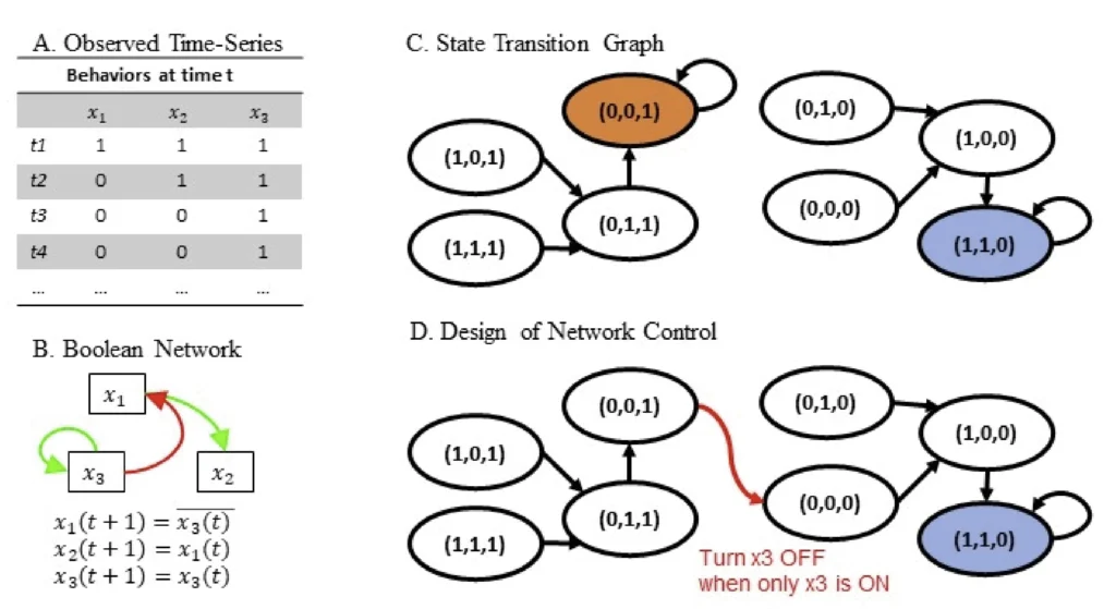
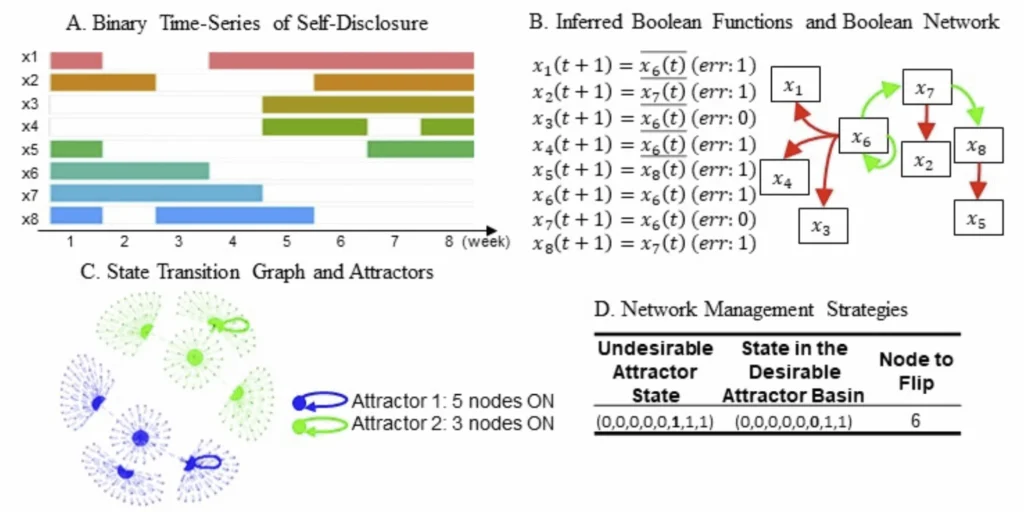
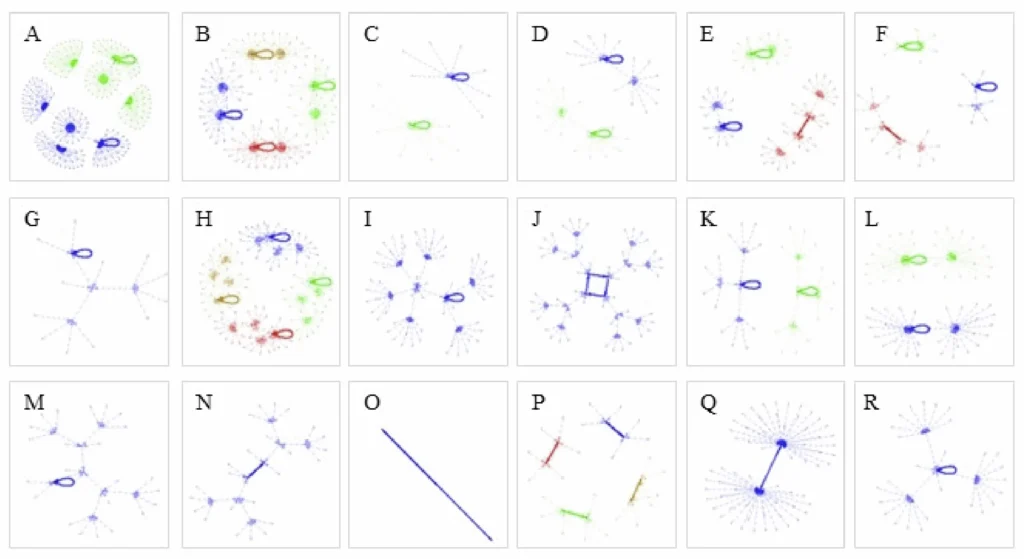
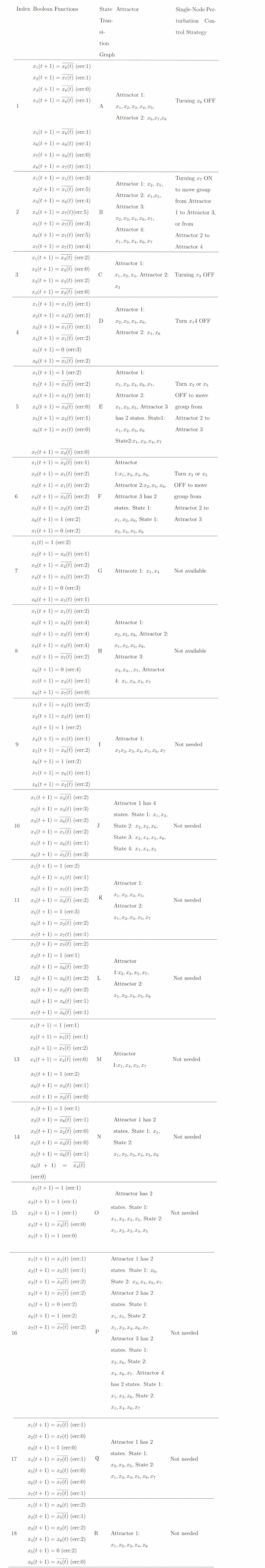
Social influence processes can induce desired or undesired behavior change in individual members of a group. Empirical modeling of group processes and the design of network-based interventions meant to promote desired behavior change is somewhat limited be-cause the models often assume that the social influence is assimilative only and that the networks are not fully connected. We introduce a Boolean network method that addresses these two limitations. In line with dynamical systems principles, temporal changes in group members’ behavior are modeled as a Boolean network that also allows for application of control theory design of group management strategies that might direct the groups to-wards desired behavior. To illustrate the utility of the method for psychology, we apply the Boolean network method to empirical data of individuals’ self-disclosure behavior in multi-week therapy groups (N = 135, 18 groups, T = 10 ∼ 16 weeks). Empirical results provide descrip-tion of each group member’s pattern of self-disclosure and social influence and identification of group-specific network control strategies that would elicit self-disclosure from the majori-ty of the group. Of the 18 group models, 16 included both assimilative and repulsive social in-fluence. Useful control strategies were not needed for 10 already well-functioning groups, were identified for 6 groups, and were not available for 2 groups. The findings illustrate the utility of the Boolean network method for modeling the simultaneous existence of assimila-tive and repulsive social influence processes in small groups, and developing strategies that may direct groups toward desired states without manipulating social ties.

Keywords: group process, social influence, Boolean network, network control, dynamical system method

  1. Northeastern University
  2. Pennsylvania State University
  3. Opinion Research Business (ORB) International
  4. Stanford University

*Please address correspondence to xiao1.yang@northeastern.edu, Departments of Health Sciences and Computer Sciences, Northeastern Uni-versity, USA

Yang, X., Albert, R., Molloy, L.E., & Ram, N. (2024). Modeling and managing behavior change in groups: A Boolean network method. advances.in/psychology, 2, e55226. https://doi.org/10.56296/aip00009

The current article passed two rounds of double-blind peer review. The anonymous review report can be found here.


Introduction

Individuals often modify their behavior according to their observation of how other individuals in their social circle behave. Individuals may choose to conform to other’s behavior because they feel safer mimicking their social peers’ behaviors (e.g., conformity, Asch, 1956; group norm, Festinger et al., 1950); or they may choose to act differently from their peers because they disagree with their peers’ behavior (Rosenbaum, 1986). Some individuals might be very consistent in their behavior and, although not changing their own behavior, might still influence their peers’ behavior (Moscovici & Zavalloni, 1969). Because social influence facilitates individuals’ behavior change in social group settings, the behavior changes among the individuals due to social influence can be conceptualized as a group process. The outcome of the group process of behavior change are often the emergence of roles, group structures, and group norms (Arrow, 2010; Nowak et al., 1990).

Theorists seeking to understand behavior change desire methods that can model social influence, and practitioners seeking to induce behavior change desire methods that can manage social influence. In this paper we introduce and forward a Boolean network method (Kauffman, 1969, 1993) that can estimate the presence of social influence and how it changes behavior within a group, and provide strategies for network management that can promote desired behavior or prevent undesired behavior. Using empirical data from a longitudinal study of self-disclosing behavior in therapy groups on college campus, we demonstrate how the Boolean network method can be applied to longitudinal behavioral data to infer social influence and to manage a group toward a desired goal – that the majority of group members will self-disclose.

Social Influence and Behavior Change in Social Groups

Theories of behavior change suggest individuals modify their behaviors according to the behaviors of their peers. There are mainly two different types of social influence regarding behavior change – assimilative and repulsive social influence (Flache et al., 2017; Stadtfeld et al., 2020). When people are under the assimilative social influence of their peers, they tend to modify their behavior to be more similar to their peers’ behavior. There are several possible mechanisms of assimilative social influence. The integrative theory of planned behavior (Yzer, 2010) suggests that perceived social norms (and social pressures to perform specific behaviors) motivate behavior change. Similarly, social learning theory suggests individuals imitate others’ behaviors through observation learning and can do so even without direct reinforcement (Bandura, 1963), and when there is uncertainty about the consequences (Bikhchandani et al., 1992). In contrast, when people are under the repulsive social influence of their social peers, they tend to modify their behavior to be different from their peers’ behavior. There are several mechanisms for repulsive social influence. First, repulsive social influence could also be social learning when a specific behavior is associated with subsequent punishment (Bandura, 1963, 1977). Second, repulsive social influence could follow from negative social ties, which refer to social ties that carry negative connotations between two persons, such as dislike (Harrigan et al., 2020; Veenstra et al., 2013). For example, if person A dislikes person B’s behavior, then person A’s behavior is more likely to move against person B’s behavior. Third, repulsive social influence may reflect dominance, particularly in groups that have limited resources (Sade & Dow, 2013). Here, group members modify their behaviors – often those related to the occupation of resources – when in the presence of a more dominant peer. For example, a less dominated group member may give up the resources voluntarily to a more dominant peer; the more dominant member can also actively fight and prevent the less dominant member from occupying resources, such as food (Senior et al., 2016), or social status (Martin, 2009). Quantitatively, the behavior of the less dominant member moves in the opposite direction of the behavior of the more dominant member, for instance, if the more dominant member occupies resources, then the less dominant member will not occupy resources.

Although many theories suggest that there are both assimilative and repulsive social influences, the methods used to model social influence on behavior change often assume that social influence is only assimilative. Prior empirical studies often examine the statistical relation between the likelihood of adopting a behavior and the number of peers that already adopted that behavior (Shameli et al., 2017; State & Adamic, 2015), positing, as per the threshold theory (Granovetter, 1978), the likelihood of adopting a novel behavior increases because the number of peers who adopted the novel behavior increases. This modeling approach assumes each dyad has assimilative social influence, so the effect of social influence on behavior from each peer can be summed up to measure the total social influence. Another modeling technique, often adopted to study the social influence on behavior change, is Simulation Investigation of Empirical Network Analysis (Snijders, 2017). Here also, the empirical applications focus heavily on the assimilative social influence in its empirical applications (Veenstra et al., 2013) through examination of the average similarity effect, total similarity effect, and average alter effect. In contrast, agent-based modeling (ABM) is a generative approach (Epstein, 1999) used to demonstrate the impact of social influence on behavior change, and it does not constrain the social influence to be only assimilative. Here, the system is modeled as multiple agents who interact with other agents according to a set of rules that can be assimilative or repulsive (e.g., copying other’s behavior or choosing the opposite behavior). Simulation is used to iteratively compute the changes in group process as agents update their behaviors based on the set of rules. Hence, ABM is often used to simulate and visualize dynamical systems to inform public health policies, but it has rarely been used to fit empirically observed behavior data (Tracy et al., 2018).

There is no theoretical reason to assume that only assimilative social influence exists in a social group; the lack of empirical studies focused on both assimilative and repulsive social influence might be due to a lack of available methods. The dynamical system method can fill this gap by estimating the dyad-level social influence based on the dyad’s social time series, without assuming the dyad-level social influence is uniform (Arrow, 2010). The dynamical system method is a mathematical model for a system’s dynamic evolution, which is typically formulated in terms of linear or nonlinear ordinary differential equations on a state-space (Kutz et al., 2016). In a dynamical system, each group member’s behavior is modeled as a set of temporal relations where the behavior at the current time is an outcome of their own and the other group members’ behavior at previous time point(s). Social influence can then be inferred from the temporal relations between each dyad in the group. For instance, when person A’s behavior at time t has a temporal relation with person B’s behavior at time t + 1, this suggests that person A’s behavior influences person B’s behavior. Depending on the direction of the temporal relation, we can infer whether it is an assimilative or repulsive social influence. For instance, when person A’s behavior at t has a positive temporal relation with person B’s behavior at t + 1, this suggests that person A’s behavior has an assimilative influence on person B’s behavior. If person B’s behavior at t has a negative temporal relation with person C’s behavior at t + 1, person B’s behavior has a repulsive influence on person C’s behavior. As such, dynamical system models can accommodate simulateneous manifestation of both assimilative and repulsive social influences within the same group. More complex dynamical system formulations might further allow for longer time lags or processes that evolved in continuous-time (Antonioni et al., 2019; van Montfort et al., 2018). In this paper, we forward a dynamical system approach using a Boolean network method that specifically models the dynamical evolution of the system from time point t to t + 1 using Boolean functions (AND, OR, NOT).

Managing the Group Process of Behavior Change

Because individuals are under social influence and likely to modify their behavior due to other group members’ behavior, the process of behavior change due to social influence in the social group context can be conceptualized as a group process of behavior change. Then there is potential to manage the group process, so that the majority of the group will adopt a desired behavior or as many group members as possible will.

Previous literature suggests managing group process can utilize social influence from the most central nodes. Acknowledging that there are other definitions of node centrality (Freeman et al., 1991; M. Newman, 2010) and much ongoing research on how centrality is related to group dynamics, degree centrality – e.g., individuals who receive the most friend nominations from others in the network – might be leveraged to prevent undesirable behavior (e.g., aggression) from being spread via the social network (Borek et al., 2019; Osgood et al., 2013). This prior work suggests that one potential group management strategy is to intervene on the peer selection process, specifically to encourage group members to affiliate with those group members who show desired behavior (e.g., no substance use) and discourage affiliation with those who show undesired behavior (e.g., substance use).

This group management strategy makes two important assumptions. The first assumption is that social influence among group members is only assimilative in a mono-layer social network with only one channel of social interactions. In multiplex networks, some channels might support assimilative social influence while others support repulsive social influence (Kivelä et al., 2014; Wasserman & Faust, 1994). When this assumption is true, those who are more central in the social network are thought to be in a position to influence more people in the group. So, positioning group members with desired behavior as the central nodes in the network should increase the number of group members that adopt desired behavior. Conversely, positioning group members with undesired behavior as fewer central nodes will allow fewer people to be influenced by them and subsequently will decrease the number of group members that adopt undesired behavior. The second important assumption underlying a centrality-based group management strategy is that the network cannot be a fully connected network, where every group member has a social tie with every other group member in the network. Only when a group is not fully connected will it be possible to manage the friend nomination so that they allow some group members to have more friend nominations than others. This assumption is valid for large networks because it is unrealistic that everyone would know everyone in a large social networks (e.g., schools, corporations, the internet). But the assumption may be invalid in small groups (e.g., therapy groups, sports teams, coauthor groups), because the small size of the group allows group members to share a social tie with every other group member.

When at least one of the two above assumptions is violated, we need a more flexible group management method. Once we can model the group process using dynamical system methods as previously introduced to relax the first assumption, we can also design network management strategies using control theory that is unconstrained by the second assumption. Control theory (or control system design), a subfield of mathematics and engineering, focuses on moving dynamic systems toward desired goals (Lewis et al., 2012; Liu & Barabasi, 2016; Molenaar & Nesselroade, 2015). For example, engineers and mathematicians have developed automated systems to direct planes to follow a designated trajectory and land at a designated lane by adjusting velocity and direction in real-time to accommodate ongoing changes in the environment (e.g., wind). Similarly, a variety of Boolean network control methods have been developed to determine the specific actions that will influence the behavior of the Boolean network so that it follows a desired trajectory or settles into a desired state (Campbell & Albert, 2019; Murrugarra et al., 2016; Shmulevich & Dougherty, 2010). In the context of group management, control theory methods focus on changing the behavior of specific group members instead of changing the social ties, which is not constrained by the second assumption about social network topology. In this paper, we will apply the Boolean network method to model the group process, and then use the network control method based on the Boolean network method to identify specific ways to manage group processes.

Boolean Network

The Boolean network method provides a realistic solution for both modeling and managing group processes for two reasons: (1) the Boolean network method does not impose the assumption that social influence is only assimilative and allows both assimilative and repulsive social influence to be modeled for the same group, and (2) the Boolean network method can provide group management strategies, even for fully connected networks, hence it can be used to design network management strategies (also called “network control”, Campbell & Albert, 2019; Murrugarra et al., 2016; Shmulevich & Dougherty, 2010), in accordance with the dynamics of social influence and without relying on manipulating social ties.

Background         

The Boolean network (BN) model was originally introduced by Kauffman (1969, 1993). In brief, a Boolean network \(G(X(t),B)\) is defined by a set of nodes \(X(t)={x_1 (t),x_2 (t),…,x_n (t)}\), where \(x_i\) is the \(i^{th}\) node, and a set of Boolean functions \(B={f_1,f_2,…,f_n}\), where each Boolean function \(f_i(x_{i1},x_{i2},…,x_{ik})\) with \(K\) specific input nodes for node \(x_i\) determines the value of \(x_i\) at time \(t+1\). In this paper, the nodes represent a group member’s behavior variable which is binary (1=ON, 0=OFF), for instance, self-disclosure behavior in a group setting. The Boolean functions represent the temporal dynamics between group members, i.e., how the group members’ behavior (nodes) influences each other’s behavior over time.

The Boolean functions are written using the Boolean operators: AND \(\land\), OR \(\lor\), NOT \(\overline{x}\). The AND (\(\land\)) operator is defined as all input variables have to be ON to turn the outcome ON; the OR (\(\lor\)) operator is defined as any input variables being ON can turn the outcome ON; the NOT (\(\overline{x}\)) operator simply takes the opposite state of the input variable. Table 1 shows how these rules produce different outcome based on the input of two variables.

Table 1

Table of input variable(s) and the outcome of AND, OR, and NOT rule

Modeling Assimilative and Repulsive Influence Simultaneously

To give an intuitive illustration of how the Boolean network method can be used to describe groups where assimilative and repulsive social influence operates simultaneously, we use a simple three-person network. Member 1, member 2, and member 3’s behaviors at multiple occasions are represented as \(x_1\), \(x_2\), and \(x_3\), respectively. The observed time-series of each person’s behavior \(x_1\), \(x_2\), and \(x_3\) are shown in Figure 1a, where the states of \(x_1\), \(x_2\), and \(x_3\) are ordered by time-steps \(t_1\), \(t_2\), \(t_3\),…. From this observed binary time series, we can infer the Boolean functions that have assimilative and repulsive social influence in the same group as follows:

\(\begin{equation} \label{eq:equation1}
x_1(t+1) = \overline{x_3(t)}\tag{1}
\end{equation}\)
\(\begin{equation} \label{eq:equation2}
x_2(t+1)=x_1(t)\tag{2}
\end{equation}\)
\(\begin{equation} \label{eq:equation3}
x_3(t+1)=x_3(t)\tag{3}
\end{equation}\)

(the details of how rules are inferred will be introduced in the Data Analysis section).

1. \(x_1(t+1)= \overline{x_3(t)}\) indicates repulsive social influence from person \(x_3\) to person \(x_1\): when \(x_3\) is OFF at time t, \(x_1\) will turn ON at time \(t+1\); when \(x_3\) is ON at time t, \(x_1\) will turn OFF at time \(t+1\). This can also be explained by dominance, member 3 dominates member 1: whenever member 3’s self-disclosure is ON at time t, member 1’s self-disclosure behavior turns OFF at time \(t+1\); when member 3’s self-disclosure is OFF at time \(t\), member 1’s self-disclosure can be ON at time \(t+1\).
2. \(x_2 (t+1)=x_1 (t)\) indicates assimilative social influence from member 1 to member 2: when \(x_1\) is ON at time t, \(x_2\) will turn ON at time \(t+1\); when \(x_1\) is OFF at time \(t\), \(x_2\) can turn OFF at time \(t+1\).
3. \(x_3(t+1)=x_3(t)\) indicates member 3’s behavior depends on him/herself: when \(x_3\) is ON at time t, \(x_3\) will continue to be ON at time \(t+1\); when \(x_3\) is OFF at time \(t\), \(x_3\) will continue to be OFF at time \(t+1\).

The Boolean functions in Equations 1 to 3 are used to construct a Boolean network, a graph of which is shown in Figure 1b. The first function “\(x_1(t+1)= \overline{x_3(t)}\)” is expressed by a red edge from \(x_3\) to \(x_1\) representing the NOT effect of \(x_3(t)\) on \(x_1(t+1)\). The second function “\(x_2(t+1)=x_1(t)\)” is indicated by a green edge from \(x_1\) to \(x_2\) representing \(x_2(t+1)\) depends on \(x_1(t)\). The third function “\(x_3(t+1)=x_3(t)\)” is indicated a green edge pointing from \(x_3\) back to itself – a self-loop. In sum, this example illustrates that a Boolean network model can have both assimilative and repulsive social influence in the same group.

Figure 1

Example of a three-node network, consisting of x1, x2, x3

Designing Network Control Without Manipulating Social Ties

Methodologically, network control focuses on modifying the state transition graph that is derived from a Boolean network. Three pieces of information need to be identified: (1) which node needs to be perturbed, (2) which states to perturb the nodes to, and (3) what is the condition to perturb the node. These three pieces of information will be useful in diagnosing when and how to drive the system (social groups or social networks) into more desirable states.

An attractor is the state (or a set of states) toward which the dynamical system approaches over time (L. Newman, 2009). We can extract attractors from the state transition graph using these Boolean functions (the details of how derivation works will be introduced in the Data Analysis section). If we represent the state of (\(x_1\), \(x_2\), \(x_3\)), e.g., (0,0,0) means all \(x_1\), \(x_2\), and \(x_3\) are OFF, we can express the state transitions as a graph, namely the state-transition graph, shown in Figure 1c. For the Boolean network in Figure 1c, where the arrows indicate the direction of transitions, the state of the system will transition from (0,0,0) to (1,0,0), and then from (1,0,0) to (1,1,0). Once the system enters (1,1,0), it will be absorbed in this state and it will not transition to other states. This kind of state, where the system stays, is an attractor.

The Boolean network method utilizes the differential desirability of attractors within the same dynamical system and designs network control strategies to move the dynamical system from an undesirable attractor to a desirable attractor, where desirability of each attractor is based on practical concerns (e.g., the common good). For instance, in our illustration, we define a desirable attractor as an attractor in which the majority of group members’ self-disclosure are ON. For example, an attractor in which two group members’ self-disclosure is ON, e.g., (1,1,0), is deemed desirable; on the contrary, an attractor in which only one group member’s self-disclosure is ON, e.g., (0,0,1), is deemed undesirable.

The control strategy can be derived based on the distance from an undesirable attractor to the basin of a desirable attractor (the details of this derivation will be introduced in the Data Analysis section). We can design network control based on the extracted attractors. One network control strategy is to perturb \(x_3\) when only \(x_3\) is ON, as shown in Figure 1d, so that the system will transition from (0,0,1) to (0,0,0) indicated by a red arrow. From there, the system will go to (1,0,0), and eventually to (1,1,0), the desirable attractor. This new state transition is also depicted in Figure 1d. In sum, this example illustrates that a Boolean network method can be used to design network management strategies based on the dynamics of social influence without relying on manipulating social ties.

The Present Study

In the present study, we model social influence processes driving week-to-week disclosure behaviors of all members of a therapy group. In doing so, we construct Boolean networks that simultaneously estimate assimilative and repulsive social influence from the Boolean functions. The assimilative social influence is shown in a function form like \(x_j(t+1)=x_i(t)\), and a repulsive social influence is shown in a function form like \(x_j(t+1)=\overline{x_i(t)}\). Then based on the Boolean network of each group, we can extract attractors for each group, and assign desirability to the attractors. When there are both desirable and undesirable attractors for the same group, we can search for a control strategy and identify specific group members that can move the group into a desirable attractor. The strength and novelty of this Boolean network method includes (a) simultaneously estimating assimilative and repulsive social influence from dynamics of group members’ behavior data, and (b) providing group management strategy by applying network control on the dynamics of group members’ behavior data.

Method

Data for our empirical inquiry are drawn from a longitudinal study of the dynamics of university counseling center therapy groups that met weekly, and how the mental health and behaviors of individuals within those groups changed over 10 to 16 weeks. A comprehensive description of the larger study can be found in Molloy (2012). Details relevant to the present analysis are given below.

Participants and Procedure

Weekly data were collected from university students (undergraduate and graduate students) receiving mental health services in the form of group therapy, from a university counseling center. Data were only collected from recruited groups in which all members (the two group leaders and all clients) had consented to participate, resulting in data from 135 individuals in 18 therapy groups (Mgroup size = 7.5, not including the therapists). The participating groups met weekly for between 10 to 16 weeks. Of the 18 groups, 17 were “general process” groups (e.g., no specific disorder or topic; 9 for undergraduate students, 8 for graduate students), and one was a substance abuse group (for both undergraduate and graduate students).

Measures

Measures for the present study were drawn from the American Group Psychotherapy Association’s (AGPA) CORE-R Battery (Clinical Outcome Results Standardized Measures, Revised; see (Burlingame et al., 2006; Strauss et al., 2008): a manual of evidence-based instruments that serve as a standardized “toolbox” for clinicians to systematically monitor and evaluate groups and their members. Since the original measures were often not administered on a weekly basis, many of the items were re-worded to be present-focused by adding, for example, the phrases “during today’s session” or “today.”

Participants’ Weekly Self-Disclosure

To demonstrate the Boolean network modeling approach, we use a self-disclosure item from the Group Evaluation Scale (GES; Hess, 1996), a seven-item measure assessing the overall benefit that a client experienced during a given session. Traditional Likert-type response scales (e.g., 1 = ’strongly disagree’ to 7 = ’strongly agree’) were converted to “touch-point continuum” (slider-type) response scales (0 to 100) with end-point anchors. The ease of self-disclosure item is measured using the prompt “During today’s session, I was able to explain my problems to other members with:” and the end-point anchors were “great difficulty” and “great ease“. To prepare the variable for analysis using the Boolean network method, the interval-scale variable was binarized separately for each individual using their person-specific mean score across the repeated measures. Specifically, responses above the person-mean were coded as = 1, and responses equal to or below the person-mean were coded as = 0 (alternatively, the person-median could be used). Thus, for each person in a group, we obtained a binary time series that is interpreted as indicating whether or not that individual engaged in self-disclosure during each session (we consider the measure of ease of self-disclosure an approximate measure of self-disclosure behavior, for more detailed discussion can be found in Limitations and Outlooks).

Data Analysis

Though concepts of complexity and dynamical system were introduced to psychologists early on (Ashby, 1947) and these concepts are closely related to the Boolean network method (Metcalf & Kauffman, 2021), empirical use of the Boolean network method in the psychology literature is very rare. To cover the essential concepts and methodological details that might enable readers gaining a solid understanding of the Boolean network method as a method for network modeling and network control, we synthesized the Boolean network method introduced in system biology literature.

The Boolean network method we introduce here has three major steps: (1) inference of Boolean functions and construction of a Boolean network, (2) extraction of attractors based on the inferred dynamics and assignment of desirability for each attractor, and (3) design of network control to direct a group toward a desired attractor and identify how the Boolean network needs to be updated. The tutorial code in R is available at https://osf.io/gxunk/.

Data Pre-processing

Missing data are imputed using R package imputeTS (Moritz & Bartz-Beielstein, 2017). The imputation method uses Kalman filter to maintain the characteristics of time series (e.g., time trend, oscillation), and the imputation is applied to every group member’s univariate time series first. Imputation requires a minimum of 3 non-missing data points for each group member. Hence, we choose to remove the group member’s data when they have only two or fewer data points.

At the level of group members, the number of missing data points is on average 3.23 (SD = 2.68). If we divide the number of missed data points by the total number of weeks for group meetings, then the proportion of missing data is on average 0.34 (SD = 0.27). The number of removed group members, those who had 2 or fewer data points, is 16 out of the 135 group members.

Inference of Boolean Functions and Construction of Boolean Network

The Boolean functions can be inferred from the observed time series of all the variables. Input variable refers to the variables that produce the outcome variable, similar to predictors. The number of input variables is usually denoted by k, and the size of the network is denoted by N, so the Boolean network with size N and with k input variables is sometimes called a NK Boolean network.

Algorithms have been developed to infer Boolean functions (Akutsu et al., 2000; Lähdesmäki et al., 2003; Steinway et al., 2016). The goal of inferring Boolean functions is to find the combination of input variables connected by the AND, OR, and NOT Boolean operators, that is the best fit of an outcome variable. The inference procedure utilized the matrix multiplication and fingerprint function (Akutsu et al., 2000) to compare the time series of the outcome variable and the time series of combinations of different input variables. The fingerprint function is a procedure that maps an arbitrarily large data item (such as a long binary time-series string in the observed time-series) to a much shorter bit string, its fingerprint, that uniquely identifies the original data for all practical purposes (Broder, 1993).

For network construction, each group member’s self-disclosure data within their group were entered in the BoolNet R package (Müssel et al., 2010) to construct a group-specific Boolean network. The R package will find the best fit for each variable – each member’s self-disclosure – at time t + 1 in the form of a Boolean function that uses the variables of the same group – group members’ self-disclosure – as input variables at time t . All the Boolean functions together comprise the Boolean network model of the given therapy group. The Boolean network is constructed by putting all the inferred Boolean functions together. As a hypothetical example, Figure 1b shows how the three-node Boolean network introduced earlier is constructed.

Selection of Number of Input Variable k

In this paper, we select k = 1, meaning each node is only predicted by one other node. The main reason for selecting k = 1 is that due to the relatively short time series (10 ∼ 16 weeks), selecting k = 1 can avoid overfitting the data. In addition, selecting k = 1 can also provide a straightforward interpretation of the group process – assimilative or repulsive – that matches more closely to the theory of social influence. From the set of possible functions, we identify the Boolean function that has the minimal error, in which error is defined as the sum of false positive predictions (type 1 error) and false negative predictions (type 2 error) (Lähdesmäki et al., 2003). Given differences in number of observations across groups, we will report the error rate (error/# of observations), in the Results section to ensure the error rate can be compared or aggregated across groups.

We also want to note there could be multiple Boolean functions that have the best fit for one variable. Hence, there are multiple combinations of Boolean functions within the group that have equal probability. Here, for the purpose of brevity, we describe the subsequent analytical steps with one selected Boolean function. The choice of the Boolean function is the first inferred Boolean function out of all best-fit Boolean functions in the output of the R package BoolNet. To explore all possible Boolean functions, researchers can go through each possible combination of Boolean functions within a group. In the Results section later, we also introduce the results of one set of selected Boolean functions.

Extraction of Attractors

After the Boolean functions are inferred, the state transition graph can be constructed by an exhaustive search of all possible state transition sequences from each initial condition (each combination of node states). The attractors are identified by constructing the state transition graph and finding each absorbing state, which is a state that will transition to itself due to the dynamics.

We will go through the same example of a three-node network to demonstrate this procedure, using the Boolean network mentioned earlier in Figure 1 and Equation 1 to Equation 3. For the 3-node network, there are \(2^N=2^3=8\) possible initial conditions: (0,0,0), (0,0,1), (0,1,0), (0,1,1), (1,0,0), (1,0,1), (1,1,0), (1,1,1). Using the Boolean functions, we can compute the state of the system for the next time point, \(t\) = 1. For example, when the system starts with initial condition at \(t\) = 0 of (0,0,0), meaning \(x_1=0\), \(x_2=0\) , \(x_3=0\) at \(t= 0\), then \(x_1(t=1)=\overline{x_3(t=0)}= 1\), \(x_2(t=1)=x_1(t=0)=0\), \(x_3(t=1)=x_3(t=0)=0\). We then know (0,0,0) will transition to (1,0,0). Similarly, we can compute the next state when the system starts at one of the other seven states. We have put the initial state and state at the next moment in Table 2.

The overall state transitions from Table 2 can be represented as a state transition graph. Shown in 1c, the states are shown as circles, and the arrows indicate the direction of change between different states. Attractors are identified as the states where the state at t + 1 is identical to the state at t. One attractor (the seventh row in Table 2, colored in light blue) is (1,1,0), having two nodes \(x_1\), \(x_2\) turned ON. The other attractor (the second row in Table 2, colored in yellow) is (0,0,1), having one node \(x_3\) turned ON.

It is worth mentioning that there are two types of attractors: the fixed-point attractor when the system stays in one state, and a complex attractor (also called a limit cycle) when the system cycles through a finite set of states. The limit cycle can be identified by analyzing the state transition graph; if there is a cycle of state transitions that returns to the starting state in the state transition graph, there is a limit cycle formed by that set of states.

Table 2

Table of state transitions

(x1, x2, x3)
tt + 1
(0,0,0)(1,0,0)
(0,0,1)(0,0,1)
(0,1,0)(1,0,0)
(0,1,1)(0,0,1)
(1,0,0)(1,1,0)
(1,0,1)(0,1,1)
(1,1,0)(1,1,0)
(1,1,1)(0,1,1)

Design of Network Control

For this paper, we aim to suggest a change to particular members’ behavior such that a therapy group will not get stuck with only a few people self-disclosing all the time, but instead elicit more diverse participation in self-disclosure. Generally speaking, self-disclosure is a desirable behavior in therapy groups because it can strengthen the therapeutic process and group members’ self-evaluation can enhance their own healing and change (Farber, 2006).

We consider a single-node perturbation to minimize the burden for group therapists, who are expected to execute the control strategy. According to network control methods (Campbell & Albert, 2019; Murrugarra et al., 2016; Shmulevich & Dougherty, 2010), we introduce how to identify three pieces of information in this section: (1) which node (i.e., person) needs to be perturbed, (2) which state to perturb node to, and (3) what is the condition to perturb the node. These three pieces of information will be useful in diagnosing when and how to drive the system into more desirable states for social groups. The procedure for identifying control strategy is as follows:

1.   Formulate the goal of network control. The goal is formulated in accordance with practical/substantive concern. For this paper, the goal is to promote the desired behavior (self-disclosure), and the desirability of attractors is determined by the number of participants whose self-disclosure is ON at least once in the attractor. The desirability of an attractor is determined by whether the majority of the group members have self-disclosure ON. Here, the method relies on the naturally occurring attractors based on the existing group dynamics, so we chose the desirable state as the majority’s self-disclosure ON if such attractor state is applicable. Ideally, it might be most desirable to have all group members self-disclose, but this kind of attractor is not guaranteed to occur in the existing group dynamics.

2.  Compute the Hamming distance from an undesirable attractor to the states in a desirable attractor basin. An attractor basin is defined as the set of states that will eventually go to a given attractor state. The attractor basin can be identified from the state transition graph; it is made up of all the states in this graph that are connected to the attractor by a state transition or a succession of state transitions. Because the system will eventually go to the attractor once the system is in any state belonging to the attractor basin, we can consider what actions are necessary to move the system from an undesirable attractor state into the basin of a desirable attractor. Ideally, we would like to move the system from an undesirable attractor state to the closest state in the desirable attractor basin. The distance from an undesirable attractor state to each state in the desirable basin will be the number of nodes that need to be perturbed, thus shortest distance indicates fewest nodes to be perturbed. Formally, these distances are computed using Hamming distance (Hamming, 1950), which compares two binary strings of equal length and counts the number of bit positions in which the two bits are different. For example, the distance between state (0,0,1) and state (1,0,0) is 2 because two elements (\(x_1\) and \(x_3\)) in the string are different, and need to be changed to move the system from one state to the other state.

3.  Formulation of control strategy. Once all of the Hamming distances are computed, we formulate control strategies from those that have the shortest distance. The Hamming distance indicates the number of nodes that need to be perturbed. So, the shortest Hamming distance indicates a control strategy with minimal number of nodes perturbed; when the shortest Hamming distance is 1, then we obtain a single-node perturbation, which is what we choose as the control strategy. The node to be perturbed is the node whose state differs between the undesirable attractor state and the state in the desirable attractor basin state. The undesirable attractor state is the condition to perturb the node, and the state in the desirable attractor basin state is the state in the node that should be perturbed to.

An example is shown in Figure 1. A three-node Boolean network and its state transition graph are given in 1b and 1c. The state transition has one desirable attractor (1,1,0) in blue and one undesirable attractor (0,0,1) in orange, because the (1,1,0) has 2 group members’ self-disclosure ON, compared with (0,0,1). The goal of network control is to move the system out of the undesirable attractor (0,0,1) and direct the system into the desirable attractor (1,1,0).

We compute the Hamming distances between the undesirable attractor (0,0,1) and every state in the attractor basin that includes the desirable attractor state (1,1,0). We then find the shortest distance, which in this case is from (0,0,1) to (0,0,0), and develop a control strategy that would facilitate that move.

Figure 1d shows the control strategy – turning node \(x_3\) OFF – that when invoked can move the system towards the desirable attractor. The node to perturb is node \(x_3\) because the undesirable attractor state (0,0,1) and the state in the desirable attractor basin that has the shortest Hamming distance (0,0,0), differing by the third node. The condition to perturb is when the system is stuck in the undesirable attractor (0,0,1), the state to perturb \(x_3\) to is to turn \(x_3\) to 0 (OFF), then the system goes to (0,0,0), and the state transition is highlighted as a red arrow in Figure 1d. From there, the system will then transition to (1,0,0), and then to the desirable attractor (1,1,0), highlighted by blue, where two group members will have the desirable behavior = ON. It is worth noting there could be multiple states that have a distance of 1 to the undesirable attractor, indicating multiple control strategies. It is also possible that there is no state that has a distance of 1 to the undesirable attractor, indicating that no single-node control strategy could be found.

Results

We used the Boolean network method to describe the group process of each of the 18 therapy groups’ self-disclosure and to design a control strategy that would move each group toward a desirable outcome – where the majority of group members engage in self-disclosure. Results are reported in two parts. First, we go step-by-step through the results obtained for an exemplar group. Then, we summarize and identify patterns in the findings across all 18 groups.

Group-Specific Analysis: Identifying a Management Strategy

In this section, we illustrate how the analyses proceeded for one exemplar group, Group 1 in Table 3. Group 1 consisted of 8 persons, \(x_1\) to \(x_8\), who participated in group therapy for 8 weeks. The self-disclosure behavior of each member is shown in Figure 2a, where the colored blocks indicate the weeks that each individual self-disclosed and the white spaces indicate the weeks they did not self-disclose.

Inference of Boolean functions and construction of Boolean networks. The Boolean functions inferred from this 8-dimensional binary time-series were, as also shown in Figure 2b,

\(\begin{equation} \label{eq:equation4}
x_1(t+1) = \overline{x_6(t)} (err:1)
\end{equation}\tag{4}\)
\(\begin{equation} \label{eq:equation5}
x_2(t+1)= \overline{x_7(t)} (err:1)
\end{equation}\tag{5}\)
\(\begin{equation} \label{eq:equation6}
x_3(t+1)= \overline{x_6(t)} (err:0)
\end{equation}\tag{6}\)
\(\begin{equation} \label{eq:equation7}
x_4(t+1) = \overline{x_6(t)} (err:1)
\end{equation}\tag{7}\)
\(\begin{equation} \label{eq:equation8}
x_5(t+1)= \overline{x_8(t)} (err:1)
\end{equation}\tag{8}\)
\(\begin{equation} \label{eq:equation9}
x_6(t+1)= x_6(t) (err:1)
\end{equation}\tag{9}\)
\(\begin{equation} \label{eq:equation10}
x_7(t+1) = x_6(t) (err:0)
\end{equation}\tag{10}\)
\(\begin{equation} \label{eq:equation11}
x_8(t+1)= x_7(t) (err:1)
\end{equation}\tag{11}\)

These functions indicate that the group process included both assimilative and repulsive social influences. Specifically, Equation 10 indicates an assimilative social influence from \(x_6\) to \(x_7\), in that \(x_7\) always does what \(x_6\) did the previous week. In contrast, Equation 4 indicates a repulsive social influence from \(x_6\) to \(x_1\), in that \(x_1\) always does the opposite of what \(x_6\) did the previous week. Collected together, the eight Boolean functions form the Boolean network for Group 1. Altogether the group process demonstrates both assimilative and repulsive social influence co-exist in the same group.

Extraction of Attractors

Based on the group-specific Boolean network, we then computed how the system evolved from t to t + 1 (e.g., as in Table 2), which is shown graphically in Figure 2c. The state transition graph in Figure 2c is obtained in the same way as introduced in the “Extraction of Attractors” section, but each state is depicted using dots in Figure 2c, instead of circles with states in Figure 1c, due to the lack of space.

Attractors – the states that transition back to themselves – can be extracted. In our example group, two attractors are identified and each attractor basin is highlighted by a different color. Attractor 1 (highlighted in blue with a loop) has five nodes (\(x_1\) to \(x_5\)) with self-disclosure = ON. Attractor 2 (highlighted in green with a loop) has three nodes (\(x_6\) to \(x_8\)) with self-disclosure ON. Based on the number of group members that have self-disclosure ON, Attractor 1 is desirable and Attractor 2 is undesirable.

Figure 2

Illustration of an eight-member group’s model results

Design of Network Control

Using the control strategy search algorithm described above we identified one strategy that might be used to move the system from Attractor 2 to Attractor 1. Hamming distance was calculated between the undesirable attractor to all states in the desirable attractor basin. Figure 2d shows there is one state that has the minimal Hamming distance – one. The node that differs from the undesirable attractor to the desirable attractor basin is node 6, or x6. These are shown in Figure 2d along with an indication of that the sixth group member x6 should be reminded to shorten the self-disclosure time so that others can self-disclose. The first row in the table indicates that when the sixth group member self-discloses (0 = OFF), the system will be moved from the state of (0,0,0,0,0,1,1,1) in Attractor 2 (3 members ON) to a state (0,0,0,0,0,0,1,1) in the desirable attractor basin, and eventually to Attractor 1 (5 members ON). In sum, this strategy indicates by turning the sixth group member OFF, the network can be moved from Attractor 2 to Attractor 1.

Between-Group Differences: Different Management Strategies

The above analysis was done for each of the 18 groups. Results are summarized in Table 3 (inferred Boolean functions, state transition graph, attractors, and control strategy) and Figure 3 (state transition graphs). As seen in the Boolean function expressions column of Table 3, each group had its own unique dynamics. All the Boolean networks were different. Thus, the state transition graphs derived from each Boolean network are unique. As seen in Figure 3, each group had a unique set of attractors, and as seen in Table 3, each group had a unique control strategy.

We did not find guidelines for a cutoff of acceptable error from the literature introducing inference of Boolean functions (Akutsu et al., 2000), so we report the empirical distribution of error in our sample. The error of inference of Boolean function for individual group member’s self-disclosure is on average 1.6 (SD = 1.1). Because each group might have a different number of observations, we use the error rate, defined as error/# of observations. Error rate of the Boolean functions for individual group member’s self-disclosure is on average 0.2 (SD = 0.09).

Figure 3

Illustration of eighteen state-transition graphs. 

Assimilative and Repulsive Social Influences

Of the 18 groups, 16 included both assimilative and repulsive social influences. Specifically, each of these groups’ Boolean functions included a function with the form of \(x_j(t+1)=x_i(t)\) which indicates assimilative social influence where \(x_j\) moves toward \(x_i\); and a function with the form of \(x_j(t+1)=\overline{x_i(t)}\) which indicates that repulsive social influence with \(x_j\) is moving away from \(x_i\). The co-existence of these Boolean functions in the same network indicates that social influence in therapy groups is not always assimilative. In all these groups it appears that some group members dominate the group discussion time and prevent other group members from participating. The other 2 groups had only repulsive social influence dynamics (Groups 14 and 15). Additionally, when a Boolean function is fixed at 0, e.g., \(x_1(t+1)=0\) that indicates the behavior of the \(i^{th}\) group member is always OFF, meaning that they never self-disclosed in the group. Such members could be conceptualized as not affected by social influence (neither assimilative or repulsive). Similarly, When a Boolean function is fixed at 1, e.g., \(x_i(t+1)=1\) that indicates the behavior of the \(i^{th}\) group member is always ON, meaning that they are committed to self-disclose every week. Such members could be conceptualized as also not affected by social influence.

Table 3

Each group’s model result, including Boolean functions, state transition graph, attractors, and control strategy (totally 18 groups)

Attractor States

The state transition graphs in Figure 3 show that 8 groups have only one attractor (state transition graph has a single color – blue, e.g., Figure 3g), and 10 groups have two or more attractors (state transition graph has multiple colors, e.g., Figure 3a). The state transition graph is obtained in the same way as introduced in the “Extraction of Attractors” section, and it is depicted using dots to represent states in Figure 3, instead of circles with states in Figure 1c, due to the lack of space. Attractors in the state transition graph are indicated by self-loops. It is worth noting that when a group has a member whose behavior is fixed at 0 or 1, the number of states in the state transition graph will reduce by half. This reduction is because only half of the initial states need to be considered in the extraction of attractor step, with one node fixed at either 0 or 1. Thus, some state transition graphs have fewer states, for instance, Figure 3o only have two states, and the corresponding Group 15 has 4 nodes being fixed at 1, and only one node x4 is free to change its state. It is also worth noting some attractors are complex attractors (or limit cycle), indicating the system cycles through a set of states, for instance, Figure 3j (or Group 10) shows an attractor with 4 states, which the system cycles through week by week.

Desirability and Number of Attractors

Based on our definition of desirability, attractors where the majority of group members’ self-disclosure is ON are considered desirable; otherwise, they are considered undesirable.

Control Strategies

Examination of the structure of groups’ attractor basins and control strategies led us to develop a typology of groups. Specifically, we identified three types of groups. These are described in Table 4. The first type is the manageable group. These groups (N = 6) had multiple attractors that had differential desirability, and a single-node perturbation control strategy was available to move the system into a more desirable attractor. The second type is the unmanageable groups. These groups (N = 2) had one or four attractors. In any attractor, the group cannot reach the majority of the group members’ self-disclosure being ON, so no single-node perturbation control strategy is available because there is no alternative desirable attractor to direct the system to. The third type is the well-functioning group. These groups (N = 10) had one, two, or four attractors, and each attractor was desirable where the majority of the group members’ self-disclosure = ON. Thus, these groups were already functioning well and no control strategy was needed.

Table 4

Three scenarios of attractors and network control strategies (18 groups in total)

IndexTypeAttractors and Network Control Strategy Count (Groups)
1Manageable groupsHas multiple attractors with at least one desirable attractor, and has at least one control strategy available (6)
2Unmanageable groupsHas one or multiple attractors, but none is desirable, so no control strategy is available (2)
3Well-functioning groupsHas one or multiple attractors, which are all desirable, hence no control strategy is needed (10)

Exploring Alternative Boolean Functions

As previously mentioned, we only introduce one set of possible Boolean functions in the Results section for the purpose of brevity. To provide a more complete picture of the empirical example, we examine thoroughly the alternative Boolean functions and their impact on control strategy. We examined all the possible Boolean functions in a combinatory fashion and ran the analytical steps, including extraction of attractors and design of network control, for each possible combination of the Boolean functions.

We also categorized the control strategies using the same principle introduced in the previous section “Control Strategies”. We find some groups can be categorized as one particular type, and some groups can be considered as having multiple types in a probabilistic manner (for details see Table 5). For Group 1, after we explored all 27 possible Boolean function combinations, we found all of them are manageable. For Group 3, after we explore all 9 possible combinations of Boolean functions, we find that three combinations are manageable (33%), one combination is not manageable (11%), and 5 combinations are well-functioning (56%). This could be interpreted as Group 3 being manageable with a probability of 33%, unmanageable with a probability of 11%, and well-functioning with a probability of 56%.

Table 5

Proportions of network control strategies per group among all possible Boolean function combinations (totally 18 groups)

IndexManageable Count (Percentage)Unmanageable Count (Percentage)Well-Functioning Count (Percentage)
127 (100%)0 (0%)0 (0%)
26 (100%)0 (0%)0 (0%)
33 (33%)1 (11%)5 (56%)
46 (100%)0 (0%)0 (0%)
58 (67%)4 (33%)0 (0%)
620 (63%)0 (0%)12 (38%)
70 (0%)2 (100%)0 (0%)
80 (0%)2 (100%)0 (0%)
90 (0%)0 (0%)12 (100%)
106 (50%)0 (0%)6 (50%)
111 (50%)0 (0%)1 (50%)
121 (2%)0 (0%)47 (98%)
130 (0%)0 (0%)16 (100%)
143 (19%)0 (0%)13 (81%)
150 (0%)0 (0%)2 (100%)
162 (33%)2 (33%)2 (33%)
1774 (15%)6 (1%)420 (84%)
180 (0%)0 (0%)4 (100%)

Discussion

In this paper, we have introduced the Boolean network as a method to model and manage group processes. The Boolean network method provides a realistic solution for both modeling and managing group processes for two reasons. First, the Boolean network method can model both assimilative and repulsive social influence and does not impose a specific kind of social influence. Second, the Boolean network method can provide group management strategies, even for social networks with both assimilative and repulsive social influence.

The utility of the Boolean network method is demonstrated through application of this method to empirical data about when individuals self-disclose in therapy groups (4 to 8 participants) over 10 to 16 consecutive weeks. In the model results, we found instances where both assimilative and repulsive social influence manifest simultaneously in the same group, and that it is often possible to design network control strategies that would ensure that the majority of group members engage in the desired behavior. The detailed introduction of the Boolean network method with the accompanied tutorial and the empirical application together contribute to our knowledge and analytical repertoire about how to model and manage group processes realistically.

Assimilative and Repulsive Social Influence

The Boolean network method allows for estimation of assimilative and repulsive social influence, because it allows simultaneous existence of both positive and negative ties between group members (Harrigan et al., 2020). Confirming our expectation that assimilative and repulsive social influence can co-exist, we indeed found empirical evidence of both assimilative and repulsive social influence within groups. As such, the empirical results demonstrate the Boolean network method can model group processes in a flexible and realistic way.

Uncovering repulsive social influence can facilitate a therapist’s understanding of the group process. If only assimilative social influence is assumed and modeled, then even though there is repulsive social influence in the group, it remains undiscovered. As introduced earlier, the underlying mechanisms of repulsive social influence could be due to negative ties (Harrigan et al., 2020; Veenstra et al., 2013), social learning of negative consequences of self-disclosure (Bandura, 1977), or dominance (Martin, 2009; Sade & Dow, 2013). Identification of the dyad that has repulsive social influence can, therefore signal to a therapist that one or more of these underlying mechanisms might exist in the group and allow intervention to target the repulsive social influence that the therapist considers harmful for the group process. For example, if the therapist considers the repulsive social influence from Member A to Member B is caused by dominance, the therapist could intervene by shortening the self-disclosure of Member A and encouraging Member B to take the opportunity to self-disclose.

Generally, we have considered the NOT operator as an indicator of repulsive social influence and used dominance, social learning, or negative ties to provide a potential explanation of why such a group process would occur. An alternative interpretation, however, is that the NOT operator implies turn-taking behavior. For example, if group member 1’s behavior at time t + 1 is predicted to be NOT group member 2’s behavior at time t, then that means when group member 2 speaks at time t, then group member 1 will not self-disclose at time t + 1, which could be interpreted as group member 1 wants to give group member 2 the opportunity to continue self-disclosure.

Network Control to Manage Group Processes

The Boolean network control method does not assume social influence is only assimilative and the network control design does not rely on manipulating social ties like previous network-based interventions. We demonstrated how the Boolean network methods allow for the identification and design of group management strategies for groups with both assimilative and repulsive social influence. The dynamical system modeling framework enables the extraction of attractors by deriving state transitions from t to t + 1 and identifying the state(s) the system moved toward and is absorbed in. As a result, the control system design is based on the extracted attractors and their differential desirability and the control design provides group management strategies, which focus on changing a few group member’s behavior. The network control design shows that even if the network is fully connected, like the therapy groups in our empirical example, the control method can still find strategies to influence the majority of the group self-disclose.

The network control method makes an assumption that the group dynamics do not change so that network control strategies (group management strategies) can be effective. If the group dynamics change, which means the Boolean functions that are used to describe social influence also change, then the attractors and their desirability might change, and subsequently, the control strategies might change.

This network control method can help group therapists manage group processes. In counseling practice, therapists can use the network control strategy to guide group therapy practice and to encourage specific group members to self-disclose when the group is stuck with only a few members self-disclosing, which is an undesirable attractor, and then the group can be moved out of the undesirable attractor and have more members self-disclose. By managing the group and allowing more group members to self-disclosure, the therapy group is expected to have more effective counseling, as self-disclosure can strengthen the therapeutic process and the self-evaluation in self-disclosure can enhance healing and change (Farber, 2006). An alternative way to use the network control is that the therapist could develop a hypothesis about group management strategies (e.g., encouraging specific group members to self-disclose) and use the Boolean network method to confirm their hypothesis.

The application of the Boolean network method is not limited to only therapy groups, nor to this particular behavior (e.g., self-disclosure). The Boolean network method can be applied to a wide range of group processes that rely on social influence. Take the prevention of substance use among adolescents as an example, the Boolean network control method can provide suggestions for schoolteachers or community stakeholders. In an adolescent social network within a school/community, the Boolean network control method could be used to identify strategies for reducing the number of adolescents that adopt substance use as a regular behavior, which corresponds to adolescents’ substance use being ON in an attractor state. The strategies will require modifying a few adolescents’ substance use behavior so that the whole social network will be moved to an attractor with fewer adolescents engaging in substance use.

Limitations and Outlooks

Controllability

The desirability of an attractor, in this paper, was defined as whether the majority of group members’ self-disclosure is ON. Hence, the prerequisite of a group having a control strategy is the group must have multiple attractors with at least one desirable attractor. We found in our empirical dataset that not all groups have multiple attractors, nor do they always have at least one desirable attractor. This indicates that some groups are not controllable with the current control system design method. Further methods to assess the controllability of a Boolean network can provide a quick evaluation of whether a network is controllable (Cheng & Qi, 2009). Furthermore, the ideal attractor might be having all group members self-disclose periodically in the group therapy context, but this kind of attractor may not exist in the naturally occurring attractor(s). It may be possible to derive a management strategy to create an attractor with all group members’ self-disclosure ON with more complex perturbation strategy than a single-node perturbation (Xiao & Dougherty, 2007). However, the practical implication of a more complex group management strategy is that it may increase the burden on the group therapist. Future research, especially regarding the implementation of group management strategies, can further explore the balance between therapist burden and optimal attractor design.

Efficiency of Attractor Extraction for Larger Networks

We presented the Boolean network method and an empirical application on modeling and controlling for dynamics of social influence. The empirical example here had the main goal to maximizing the diversity of participation in group dialogue. The size of the network in the empirical example is relatively small (4 to 8), and some social networks are much larger, ranging from a classroom or school to online social networks. The large size of the network will create a challenge for attractor extraction, as it requires enumeration of all initial conditions, which is at the scale of 2n, and n is the network size (Liu & Barabasi, 2016). Methods that identify specific network structures (e.g., stable motif) can efficiently extract attractors that are needed and will facilitate controlling the dynamics of large networks (Zanudo & Albert, 2015).

Complex Social Influence

In this paper, we preselect the number of input variables included in each Boolean function as \(k\) = 1 for the purpose of not overfitting short time series and matching the theory about assimilative and repulsive social influence. When we have more observations in the time series, we can fit more complex social influence, e.g., \(k\) = 2. This has the advantage of allowing the modeling of complex social influence in a multi-person group setting. For example, if two persons team up and dominate a third person, it can be modeled using \(k\) = 2, and the Boolean function will be in the form of \(x_3(t+1)=\overline{x_1(t) \land x_2(t)}\), meaning only when both \(x_1\) and \(x_2\) are ON – occupying resources, \(x_3\) will be turned OFF – not occupying resources. To understand complex social influence, we also need theories about social influence to pinpoint specific forms and mechanisms of social influence.

Binarization of Time-Series

In our data pre-processing, we chose to binarize the time-series for each individual based on the mean as the threshold. This choice was made to introduce the Boolean network method in a straightforward and succinct manner. As noted in previous research on gene expressions (Berestovsky & Nakhleh, 2012; Hopfensitz et al., 2012), using different methods to binarize the time series might lead to discovery of different group dynamics. Future research in social dynamics applications is needed to evaluate the robustness of the network estimation based on various binarization choices.

Longer Memory of Group Process

In this paper, we focused on the temporal relation from t to t + 1 to model the group process (i.e., lag-1 relations). In reality, social systems might have longer memory than one time step, which was one week in our empirical example. Future research might look to incorporate longer time lags in the Boolean network method and evaluate if and how the proper number of lags influences the group dynamics.

Heterogeneity in Group Boolean Networks

Even though the Boolean functions we considered were relatively simple (e.g., Boolean functions with k = 1 input), We obtained a wide variety of Boolean networks, as summarized in Table 3, and substantial heterogeneity in the state-transition graphs, as shown in Figure 3. The number of possible states in a state-transition graph (the dots in the state-transition graph) is primarily determined by the size of the group. Groups of size N will have 2N possible states. Larger groups have larger number of possible states compared to smaller groups. For example, as seen in 3, group A had 8 members, and group C had 4 members, group A has more states than that of group C. Even for same-sized groups, the Boolean functions describing the dynamics may differ, and estimation of those functions could be influenced by the level of noise in the system and/or data preparation choices. In sum, we should expect heterogeneity and future research can examine all the various methodological and substantive phenomena contributing to the observed differences in group dynamics.

Peer Selection

In this study, we did not consider the process of peer selection also because we assumed that no peer selection (such as befriending or ending friendships with certain group members) occurs that would impact the effect of social influence on self-disclosure in the therapy group setting. For social influence problem that is intertwined with peer selection, more sophisticated model, such as stochastic actor-based models (Snijders et al., 2010), are needed to properly model group processes. A stochastic actor-based model that can model peer selection as well as peer influence while allowing the social influence to be assimilative or repulsive would be an ideal model framework.

Empirical Example

The participants in this paper were young adults, and for privacy reasons, their demographic information and severity of psychopathology were not included in the analyses. Before generalizing to larger populations, it will be useful to test this approach with other populations, including individuals with various degrees of psychopathology, and with both younger and older individuals. In terms of variables, we selected the item about self-disclosure over some of the other weekly measures of participant “progress” (e.g., self-efficacy), because self-disclosure is more easily observed by other group members, and thus has the potential to generate social influence in the process of group therapy. A caveat with this measure is that the exact survey item was the ease of self-disclosure, which may differ from whether a participant did or did not self-disclosure. For lack of a more precise measure of self-disclosure behavior, we use ease of self-disclosure as a proxy of self-disclosure behavior. Another caveat of using self-disclosure to model social influence is that self-disclosure may be dependent on social desirability (Anchor et al., 1972) and can alter or unify self-disclosure behavior and consequent attractor states (e.g., high proportion of individuals’ self-disclosure being ON/OFF). This implies that groups that have more individuals with higher social desirability might have a different group dynamic than the groups that have fewer individuals with higher social desirability. Given the heterogeneity in the Boolean networks across different groups, it maybe useful to examine the relation between social desirability and group dynamics. The measurement in our dataset of self-disclosure behavior has 10 ∼ 16 weeks/observations, and this is often considered a short time series for dynamical system models. To avoid overfitting the data, we selected the number of input variables k = 1. For more complex social influence, involving a higher number of input variables, more repeated measures of behavior data would be needed. Longer measurements of behavior data would be helpful to improve the precision of analysis and identify more complex social influences.

Conclusion

In this paper, we introduced the Boolean network method as a method to model and manage group processes. To demonstrate the utility of this method, we applied this method on an empirical dataset, focusing on managing self-disclosure behavior in group therapy settings. Our modeling approach addresses gaps in previous network-based intervention literature through construction of networks that simultaneously accommodate both assimilative and repulsive social influence, and that allow for design of network control strategies for networks in which both types of social influence dynamics are operating. The Boolean network method is a more flexible, realistic, and precise method to design network-based intervention. We hope that this first application and demonstration of Boolean networks to repeated measurement of fully connected groups will open up discussions and invite more empirical studies of network control system design for social networks.

Conflicts of Interest

The authors declare no conflicts of interest.

Acknowledgments

Thanks very much to the study participants for providing a detailed glimpse of their behavior dynamics, and to the many research assistants who collect the data. This work was supported by the National Institute on Health (R01 HD076994, T32 AG049676) and the Penn State Social Science Research Institute. Please note that the present thesis was based on the unpublished PhD dissertation of the first author.

Author Contributions

Y.X., and R.N. designed the study, M-E.L. collected the data. Y.X. analyzed the data and wrote up the results. Y.X., and R.N. drafted the introduction, methods, and discussion sections. All authors provided critical revisions.

References

Akutsu, T., Miyano, S., & Kuhara, S. (2000). Algorithms for identifying Boolean networks and related biological networks based on matrix multiplication and fingerprint function. Journal of Computational Biology, 7(3-4), 331-343. https://doi.org/10.1089/106652700750050817

Anchor, K. N., Vojtisek, J. E., & Berger, S. E. (1972). Social desirability as a predictor of self-disclosure in groups. Psychotherapy: Theory, Research Practice, 9, 262–264. https://doi.org/10.1037/h0086763 

Antonioni, A., Martinez-Vaquero, L. A., Mathis, C., Peel, L., & Stella, M. (2019). Individual perception dynamics in drunk games. Physical Review E, 99(5), 052311. https://doi.org/10.1103/PhysRevE.99.052311 

Arrow, H. (2010). Dynamical system approach. In J. Levine & M. Hogg (Eds.), Encyclopedia of group processes and intergroup relations (pp. 232–234). Sage Publications.

Asch, S. E. (1956). Studies of independence and conformity: I. A minority of one against a unanimous majority. Psychological Monographs: General and Applied, 70 (9), 1–70. https://psycnet.apa.org/doi/10.1037/h009378

Ashby, W. R. (1947). Principles of the self-organizing dynamic system. Journal of General Psychology, 37, 125–128. https://doi.org/10.1080/00221309.1947.9918144

Bandura, A. (1963). Social learning and personality development. Holt, Rinehart, Winston.

Bandura, A. (1977). Social learning theory. General Learning Press.

Berestovsky, N., & Nakhleh, L. (2012). An evaluation of methods for inferring Boolean networks from time-series data. PLoS ONE, 8, e66031. https://doi.org/10.1371/journal.pone.0066031

Bikhchandani, S., Hirshleifer, D., & Welch, I. (1992). A theory of fads, fashion, custom, and cultural change as informational cascades. Journal of Political Economy, 100 (5), 992–1026. https://doi.org/10.1086/261849

Borek, A. J., Abraham, C., Greaves, C. J., Gillison, F., Tarrant, M., Morgan-Trimmer, S., McCabe, R., & Smith, J. R. (2019). Identifying change processes in group-based health behaviour-change interventions: development of the mechanisms of action in group-based interventions (MAGI) framework. Health Psychology Review, 13(3), 227-247. https://doi.org/10.1080/17437199.2019.162528

Broder, A. Z. (1993). Some applications of Rabin’s fingerprinting method. In R. Capocelli, A. DeSantis, & U. Vaccaro (Eds.), Sequences ii: Methods in communications, security, and computer science (pp. 143–152). Springer-Verlag. https://doi.org/10.1007/978-1-4613-9323-8_11

Burlingame, G., Strauss, B., Joyce, A., McNair-Semands, R., MacKanzie, K., Ogrodniczuk, J., & Taylor, S. (2006). Core battery-revised: An assessment tool kit for promoting optimal group selection, process and outcome. American Group Psychotherapy Association.

Campbell, C., & Albert, R. (2019). Edgetic perturbations to eliminate fixed-point attractors in Boolean regulatory networks. Chaos, 29 (2), 023130. https://doi.org/10.1063/1.5083060

Cheng, D., & Qi, H. (2009). Controllability and observability of Boolean control networks. Automatica, 45 (7), 1659-1667. https://doi.org/10.1016/j.automatica.2009.03.006

Epstein, J. M. (1999). Agent-based computational models and generative social science. Complexity, 4, 41-60. https://doi.org/10.1002/(SICI)1099-0526(199905/06)4:5<41::AID-CPLX9>3.3.CO;2-6

Farber, B. (2006). Self-disclosure in psychotherapy. Guilford Press.

Festinger, L., Schachter, S., & Back, K. (1950). Social pressures in informal groups. Stanford University Press.

Flache, A., Mas, M., Feliciani, T., Chattoe-Brown, E., Deffuant, G., Huet, S., & Lorenz, J. (2017). Models of social influence: Towards the next frontiers. Journal of Artificial Societies and Social Simulation, 20 (4), 2. https://doi.org/10.18564/jasss.3521

Freeman, L. C., & Borgatti, S.P. and White, D. R. (1991). Centrality in valued graphs: A measure of betweenness based on network flow. Social Networks, 13, 141-154. https://doi.org/10.1016/0378-8733(91)90017-N

Granovetter, M. (1978). Threshold models of collective behavior. American Journal of Sociology, 83 (May), 489-515. https://doi.org/10.1086/226707

Hamming, R. W. (1950). Error detecting and error correcting codes. The Bell System Technical Journal, 29 (2), 147-160. https://doi.org/10.1002/j.1538-7305.1950.tb00463.x

Harrigan, N. M., Labianca, G., & Agneessens, F. (2020). Negative ties and signed graphs research: Stimulating research on dissociative forces in social networks. Social Networks, 60, 1-10. https://doi.org/10.1016/j.socnet.2019.09.004

Hess, H. (1996). Zwei Verfahren zur Einschätzung der Wirksamkeit von Gruppenpsychotherapie. In B. Strauss, J. Eckert, & V. Tschuschke (Eds.), Methoden der empirischen Gruppentherapieforschung-ein Handbuch (pp. 142-158). VS Verlag für Sozialwissenschaften Wiesbaden. https://doi.org/10.1007/978-3-663-10786-6_10

Hopfensitz, M., Mussel, C., Wawra, C., Maucher, M., Kuhl, M., Neumann, H., & Kestler, H. (2012). Multiscale binarization of gene expression data for reconstructing boolean networks. IEEE/ACM Transactions on Computational Biology and Bioinformatics, 9, 487-498. https://doi.org/10.1109/TCBB.2011.62

Kauffman, S. (1969). Metabolic stability and epigenesis in randomly constructed genetic nets. Journal of Theoretical Biology, 22, 437-467. https://doi.org/10.1016/0022-5193(69)90015-0

Kauffman, S. (1993). The origins of order: Self-organization and selection in evolution. Oxford University Press. https://doi.org/10.1093/oso/9780195079517.001.0001

Kivelä, M., Arenas, A., Barthelemy, M., Gleeson, J. P., Moreno, Y., & Porter, M. A. (2014). Multilayer networks. Journal of Complex Networks, 2, 203-271. https://doi.org/10.1093/comnet/cnu016

Kutz, J., Brunton, S., Brunton, B., & Proctor, J. (2016). Dynamic mode decomposition: Data-driven modeling of complex systems. Society for Industrial & Applied Mathematics. https://doi.org/10.1137/1.9781611974508

Lähdesmäki, H., Shmulevich, I., & Yli-Harja, O. (2003). On learning gene regulatory networks under the Boolean network model. Machine Learning, 52 (1), 147-167. https://doi.org/10.1023/A:1023905711304

Lewis, F. L., Vrabie, D. L., & Syrmos, V. L. (2012). Optimal control. John Wiley Sons. https://doi.org/10.1002/9781118122631

Liu, Y., & Barabasi, A. (2016). Control principles of complex networks. Reviews of Modern Physics, 88 (3), 3-58.

Martin, J. L. (2009). Formation and stabilization of vertical hierarchies among adolescents: Toward a quantitative ethology of dominance among humans. Social Psychology Quarterly, 72 (3), 241-264. https://doi.org/10.1177/019027250907200307

Metcalf, G., & Kauffman, S. (2021). Systems science, cybernetics, and complexity. In G. S. Metcalf, K. Kijima, & H. Deguchi (Eds.), Handbook of systems sciences (pp. 1-35). Springer. https://doi.org/10.1007/978-981-15-0720-5_67

Molenaar, P., & Nesselroade, J. (2015). Systems methods for developmental research. In R. Lerner (Ed.), Handbook of child psychology and developmental science (pp. 652–682). Wiley. https://doi.org/10.1002/9781118963418.childpsy117

Molloy, L. E. (2012). A within-network variability approach to understanding “process” in group-based interventions (order no. 3569236). Available from ProQuest Dissertations Theses AI. (1348182275).

Moritz, S., & Bartz-Beielstein, T. (2017). Imputets: Time series missing value imputation in R. The R Journal, 9 (1), 207-218. https://doi.org/10.32614/RJ-2017-009

Moscovici, S., & Zavalloni, M. (1969). The group as a polarizer of attitudes. Journal of Personality and Social Psychology, 12 (2), 125-135. https://doi.org/10.1037/h0027568

Murrugarra, D., Veliz-Cuba, A., Aguilar, B., & Laubenbacher, R. (2016). Identification of control targets in Boolean molecular network models via computational algebra. BMC Systems Biology, 10 (1), 94. https://doi.org/10.1186/s12918-016-0332-x

Müssel, C., Hopfensitz, M., & Kestler, H. (2010). Boolnet – an R package for generation, reconstruction, and analysis of Boolean networks. Bioinformatics, 26 (10), 1378-1380. https://doi.org/10.1093/bioinformatics/btq124

Newman, L. (2009). Human-environment interactions: Complex systems approaches for dynamic sustainable development. In R. Meyers (Ed.), Encyclopedia of complexity and systems science (pp. 4631-4643). Springer. https://doi.org/10.1007/978-0-387-30440-3_273

Newman, M. (2010). Networks: An introduction. Oxford University Press. https://doi.org/10.1093/acprof:oso/9780199206650.003.0001

Nowak, A., Szamrej, J., & Latané, B. (1990). From private attitude to public opinion: A dynamic theory of social impact. Psychological Review, 97(3), 362-376. https://doi.org/10.1037/0033-295X.97.3.362

Osgood, D., Feinberg, M., Gest, S., Moody, J., Ragan, D., Spoth, R., Greenberg, M., & Redmon, C. (2013). Effects of prosper on the influence potential of prosocial versus antisocial youth in adolescent friendship networks. Journal of Adolescent Health, 53 (2), 174-179. https://doi.org/10.1016/j.jadohealth.2013.02.013

Rosenbaum, M. E. (1986). The repulsion hypothesis: On the nondevelopment of relationships. Journal of Personality and Social Psychology, 51(6), 1156-1166. https://doi.org/10.1037/0022-3514.51.6.1156

Sade, D. S., & Dow, M. M. (2013). Primate social networks. In S. Wasserman & J. Galaskiewicz (Eds.), Advances in social network analysis: Research in the social and behavioral sciences (pp. 152-166). Sage Publications. https://doi.org/10.4135/9781452243528.n6

Senior, A., Lihoreau, M., Buhl, J., Raubenheimer, D., & Simpson, S. (2016). Social network analysis and nutritional behavior: An integrated modeling approach. Frontiers in Psychology, 7, 18. https://doi.org/10.3389/fpsyg.2016.00018

Shameli, A., Althoff, T., Saberi, A., & Leskovec, J. (2017). How gamification affects physical activity: Large-scale analysis of walking challenges in a mobile application. Proceedings International World Wide Web Conference, 455-463. https://doi.org/10.1145/3041021.3054172

Shmulevich, I., & Dougherty, E. (2010). Probabilistic Boolean networks: The modeling and control of gene regulatory networks. Society for Industrial and Applied Mathematics. https://doi.org/10.1137/1.9780898717631

Snijders, T. A. B., van de Bunt G. G., & Steglich, C. (2010). Introduction to stochastic actor-based models for network dynamics. Social Networks, 32, 44-60. https://doi.org/10.1016/j.socnet.2009.02.004

Snijders, T. A. B. (2017). Stochastic actor-oriented models for network dynamics. Annual Review of Statistics and Its Application, 4, 342-363. https://doi.org/10.1146/annurev-statistics-060116-054035

Stadtfeld, C., Takacs, K., & Voros, A. (2020). The emergence and stability of groups in social networks. Social Networks, 60 (4), 129-145. https://doi.org/10.1016/j.socnet.2019.10.008

State, B., & Adamic, L. (2015). The diffusion of support in an online social movement: Evidence from the adoption of equal-sign profile pictures. CSCW ’15 Proceedings of the 18th ACM Conference on Computer Supported Cooperative Work Social Computing, 1741-1750. https://doi.org/10.1145/2675133.2675290

Steinway, S., Biggs, M., Loughran, T. P. Jr,, Papin, J., & Albert, R. (2016). Inference of network dynamics and metabolic interactions in the gut microbiome. PLoS Computational Biology, 11(6), e1004338. https://doi.org/10.1371/journal.pcbi.1004338

Strauss, B., Burlingam, G., & Bormann, B. (2008). Using the core-R battery in group psychotherapy. Journal of Clinical Psychology, 64(11), 1225-1237. https://doi.org/10.1002/jclp.20535

Tracy, M., Cerda, M., & Keyes, K. M. (2018). Agent-based modeling in public health: Current applications and future directions. Annual Review of Public Health, 39, 77-94. https://doi.org/10.1146/annurev-publhealth-040617-014317

van Montfort, K., Oud, J., & Voelkle, M. (2018). Continuous time modeling in the behavioral and related sciences. Springer. https://doi.org/10.1007/978-3-319-77219-6

Veenstra, R., Dijkstra, J., Steglich, C., & Van Zalk, M. (2013). Network-behavior dynamics. Journal of Research on Adolescence, 23 (3), 399-412. https://doi.org/10.1111/jora.12070

Wasserman, S., & Faust, K. (1994). Social network analysis: Methods and applications. Cambridge University Press. https://doi.org/10.1017/CBO9780511815478

Xiao, Y., & Dougherty, E. (2007). The impact of function perturbations in Boolean networks. Bioinformatics, 23, 1265-1273. https://doi.org/10.1093/bioinformatics/btm093

Yzer, M. (2010). The integrative model of behavioral prediction as a tool for designing health messages. In H. Cho (Ed.), Designing messages for health communication campaigns (pp. 21-40). Sage.

Zanudo, J., & Albert, R. (2015). Cell fate programming by control of intracellular network dynamics. PLOS Computational Biology, 11 (12), e1004672. https://doi.org/10.1371/journal.pcbi.1004672